Week 9 - FVM Literature Review

Finite volume method (FVM);

It is a method for representing and evaluating PDE's in the form of algebraic equations. In the finite volume method, volume integrals in a partial differential equation that contain a divergence term are converted to surface integral using the divergence theorem.

DIfference B/W FVM & FDM

FVM	FDM
Discretization is based upon the differential form of the PDE to be solved.	Discretization is based upon an integral form of the PDE to be solved.
Each derivative is replaced with an approximate difference formula.	The PDE is written in a form which can be solved for a given finite volum.
The computational domain is usually divided into hexahedral cells , and the solution will be obtained at each nodal point.	The computational domain is discretized into finite volumes and then for every volume the governing equations are solved.
The discretization results in a system of equation of the variable at nodal points, and once a solution is found, then we have a discrete representation of the solution.	The resulting approximate solution is a discrete, but the variables are typically placed at cell centers rather than at nodal points.

Need for interpolation and flux limiters in FVM

• The Gauss or divergence theorem states that the outward flux of a vector field through a closed surface is equal to the volume integral of the divergence over the region inside the surface.
• It is used to convert volume integrals appearing in the governing equation into surface integrals.
• The face values appearing in the convective and diffusive fluxes have to be computed by some form of interpolation from the centroid values of the control volume at both sides of the face.
• After special discretization , we can proceed with temporal discretization. By proceeding in this way we are using Method Of Lines (MOL) technique.
• The main advantage of MOL technique is that it allows us to select numerical approximations of different accuracies for the specila and temporal terms. Each term can be treated differently to yield to different accuracies.
• Nearly all flows in nature and industrial applications are unsteady. This is due to factors like instability,chemical reactions, turbulace, buoyancy, etc.

Flux Limiters

Flux limiters are used in high resolution schemes that are used to solve problems in science and engineering, particularly in CFD's described by PDE's.They are used high resolution scheme such as MUSCL to avoid wiggles that would otherwise occure with high order spatial discretization scheme due to shocks,discontinuities or sharp changes in the domain. Use of flux limiters together with an appropriate high resolution schemes make the solution Total Variation Diminishing (TVD).

The main idea behind the construction of flux limiters is to limit the spatial derivatives to realistic values for scientific and engineering problems They only come into operation when sharp wavefronts are present.For smoothly changing waves the flux limiters do not operate,and spatial derivatives can be represented by high order approximation without introducing sporious oscillations.

Interpolation schemes

It is a process to estimate the values at unknown points by using the points with known value and sample points on either side of unknown points .In FVM interpolation schemes are used to find the values of volume intergrals required at the points other than nodes.

Different types of interpolation schmes are:

• Upward interpolation scheme (UDS)
• Linear interpolation scheme
• Quadratic upwind interpolation scheme
• Hybrid interpolation scheme
• Total variation diminishing scheme
• Essential non-oscillatory interpolation scheme

1D linear heat conduction equation

1. n = 20 plot

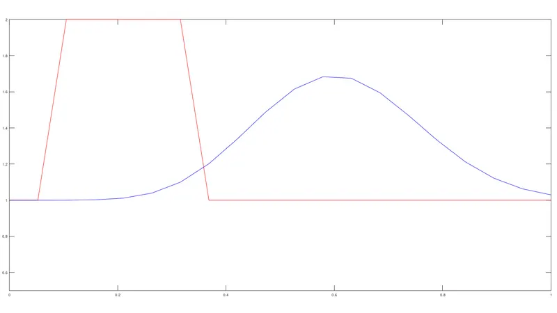
This is a velocity v/s length graph we can see that there is a drastic decrease in velocity profile. The amplitude of velocity keeps decreasing with lenght.

2. n = 40

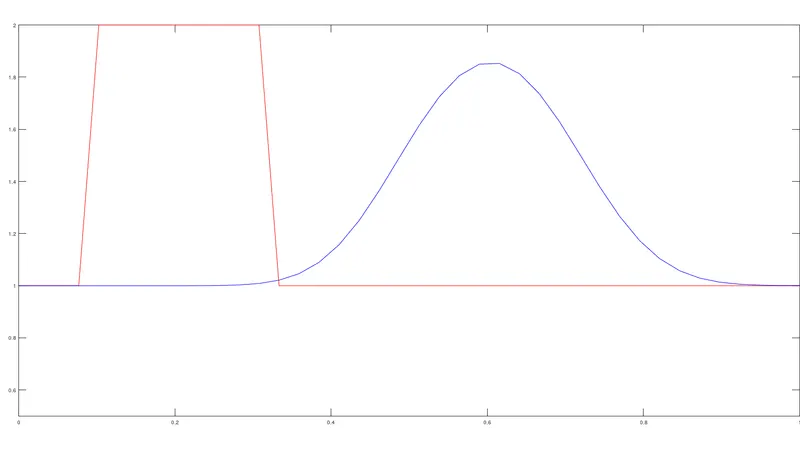
Here , there is a significant decrease in velocity profile. The truncated part is little compared to the previous graph. The amplitude of the velocity profile keeps decresing with length.

3. n = 80

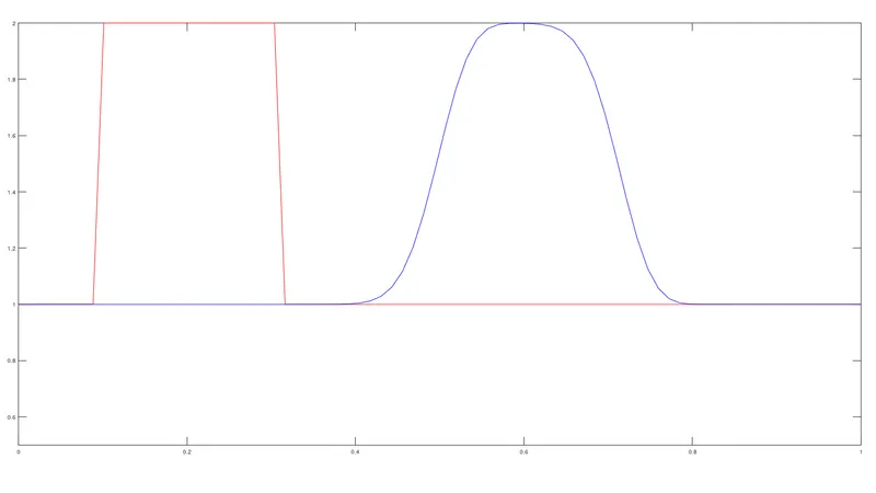
Here, there is a gradual decrease in velocity profile . The amplitude here is almost constant.

4. n = 160

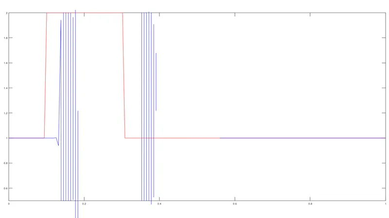
There is a disturbance in velocity profile by observing the blow up and the ripples that are formed making the graph ustable.

Comparision of the effect of time step on numerical solution

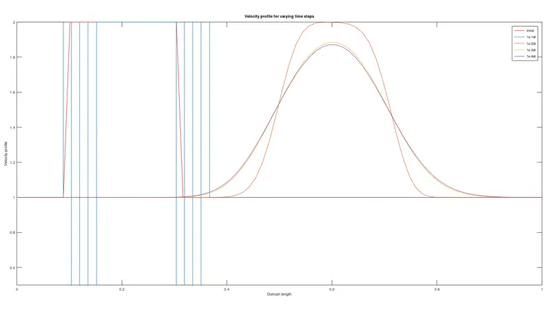
We can see that the first time step is blowing out implying that the solution is ustable . To correct this the time step value has to be corrected or within the vuable range of the solution. This can be determined by CFL condition. It is a necessary condition for convergence while solving certain PDE's.