Week 3.5 - Deriving 4th order approximation of a 2nd order derivative using Taylor Table method

Objective & aim

To derive 4th order approximation using taylor table method of function exp(x)*cos(x) in 3 methods

1.Right skewed scheme

2.Left skewed scheme

3.Central differencing

Formulation of taylor table method for right skewed scheme

`f''(x)=(af(x)+bf(x+h)+cf(x+2h)+df(x+3h)+ef(x+4h)+ff(x+5h))/h^2`

	`f(x)`	`f'(x)Deltax`	`f''(x)Deltax^2`	`f'''(x)Deltax^3`	`f''''(x)Deltax^4`	`f'''''(x)Deltax^5`
`af(i)`	a	0	0	0	0	0
`bf(i+1)`	b	b	b/2	b/6	b/24	b/120
`cf(i+2)`	c	2c	2c	4c/3	2c/3	4c/15
`df(i+3)`	d	3d	9d/2	9d/2	27d/8	81d/40
`ef(i+4)`	e	4e	8e/2	32e/3	32e/3	128e/15
`ff(i+5)`	f	5f	25f/2	125f/6	625f/24	625f/24
∑	0	0	1	0	0	0

Formulation of taylor table method for left skewed scheme

`f''(x) = (af(x)+bf(x-h)+cf(x-2h)+df(x-3h)+ef(x-4h)+ff(x-5h))/h^2`

	`f(x)`	`f'(x)Deltax`	`f''(x)Deltax^2`	`f'''(x)Deltax^3`	`f''''(x)Deltax^4`	`f'''''(x)Deltax^5`
`af(i)`	a	0	0	0	0	0
`bf(i-1)`	b	-b	b/2	-b/6	b/24	-b/120
`cf(i-2)`	c	-2c	2c	-4c/3	2c/3	-4c/15
`df(i-3)`	d	-3d	9d/2	-9d/2	27d/8	-81d/40
`ef(i-4)`	e	-4e	8e/2	-32e/3	32e/3	-128e/15
`ff(i-5)`	f	-5f	25f/2	-125f/6	625f/24	-625f/24
∑	0	0	1	0	0	0

Formulation of central differencing scheme

`f''(x)=(af(x-2h)+bf(x-h)+cf(x)+df(x+h)+ef(x+2h))/h^2`

	`f(x)`	`f'(x)Deltax`	`f''(x)Deltax^2`	`f'''(x)Deltax^3`	`f''''(x)Deltax^4`
`af(i-2)`	a	-2a	4a/2	-8a/2	16a/24
`bf(i-1)`	b	-b	b/2	-b/6	b/24
`cf(i)`	c	0	0	0	0
`df(i+1)`	d	d	d/2	d/6	d/24
`ef(i+2)`	e	-2e	4e/2	8e/2	16e/24
∑	0	0	1	0	0

clear all 
close all
clc

% right skewed matrix
A = [1 1 1 1 1 1; 0 1 2 3 4 5; 0 1/2 2 9/2 8 25/2; 0 1/6 4/3 9/2 32/3 125/6; 0 1/24 2/3 27/8 32/3 625/24; 0 1/120 4/15 81/40 128/15 625/24]

B =[0; 0; 1; 0; 0; 0]

R = inv(A)*B

% left skewed matrix
M = [1 1 1 1 1 1; 0 -1 -2 -3 -4 -5; 0 1/2 2 9/2 8 25/2; 0 -1/6 -4/3 -9/2 -32/3 -125/6; 0 1/24 2/3 27/8 32/3 625/24; 0 -1/120 -4/15 -81/40 -128/15 -625/24]

N =[0; 0; 1; 0; 0; 0]

L = inv(M)*N

% central differencing
P = [1 1 1 1 1;-2 -1 0 1 2;4/2 1/2 0 1/2 4/2;-8/2 -1/6 0 1/6 8/2;16/24 1/24 0 1/24 16/24 ]

Q = [0; 0; 1; 0; 0]

C = inv(P)*Q

x = pi/3
dx = linspace(pi/4000,pi/40,100)

% function = e^x*cos(x)
% analytical first derivative = e^x*cos(x) - e^x*sin(x)

% analytical second derivative = -2*e^x*cos(x)
analytical_derivative = -2*exp(x)*sin(x)

% function handle 
f = @(x) exp(x).*cos(x)

right_skewed_scheme = (R(1)*f(x) + R(2)*f(x+dx) + R(3)*f(x+(2*dx)) + R(4)*f(x+(3*dx)) + R(5)*f(x+(4*dx)) + R(6)*f(x+(5*dx)))./dx.^2
left_skewed_scheme = (R(1)*f(x) + R(2)*f(x-dx) + R(3)*f(x-(2*dx)) + R(4)*f(x-(3*dx)) + R(5)*f(x-(4*dx)) + R(6)*f(x-(5*dx)))./dx.^2
central_differencing = (C(1)*f(x-(2*dx)) + C(2)*f(x-dx) + C(3)*f(x) + C(4)*f(x+dx) + C(5)*f(x+(2*dx)))./dx.^2


error_right_skewed_matrix = abs(right_skewed_scheme - analytical_derivative)
error_left_skewed_matrix = abs(left_skewed_scheme - analytical_derivative)
error_central_differencing = abs(central_differencing - analytical_derivative)


figure(1)
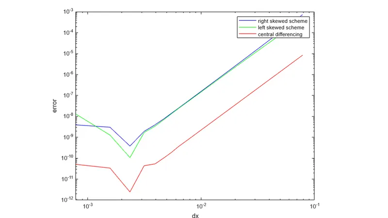
loglog(dx,error_right_skewed_matrix,'b',dx,error_left_skewed_matrix,'g',dx,error_central_differencing,'r')
xlabel('dx')
ylabel('error')
legend('right skewed scheme','left skewed scheme','central differencing')

Why is skew scheme useful ?

Result

Conclusion

As we see from the above graph the CD method has less compared to the other methods.Hence we can conclude that CD method is the most accurate than the skewed method.