Week 5.1 - Mid term project - Solving the steady and unsteady 2D heat conduction problem
To write the code which solves the 2D heat conduction equation by using the iterative methods given below ;
1.Jacobi
2.Gauss Seidel
3.Successive over relaxation
The above 3 equations can be solved in 2 ways
1.Implicit method
2.Explicit method
The given boundary conditions and values are
Top boundary = 600k
Bottom boundary = 900k
Left boundary = 400k
Right boundary = 800k
The absolute error criteria given is 1e-4
The code for 2D steady state heat equation is as given below
close all
clear all
clc

% steady state heat conduction equation d^2T/dx^2 + d^2T/dy^2 = 0

nx = 10
ny = 10

T = ones(nx,ny)

% temperatures
TL = 400
TR = 800
TT = 600
TB = 900

% Boundary conditions
T(:,1) = TL
T(:,ny) = TR
T(1,:) = TT
T(nx,:) = TB

% Edge refinement
T(1,1) = 0.5*(T(2,1) + T(1,2))
T(nx,1) = 0.5*(T(nx-1,1) + T(nx,2))
T(nx,ny) = 0.5*(T(nx-1,ny) + T(nx,ny-1))
T(1,ny) = 0.5*(T(2,ny) + T(1,ny-1))


Told = T
T_initial = T

% iterative solver =
% Jacobi

error = 9e9
tol = 1e-4

jac_iter = 0

while(error > tol)

for i = 2:nx-1
  for j = 2:ny-1

    T(i,j) = 0.25*(Told(i+1,j) + Told(i-1,j) + Told(i,j-1) + Told(i,j+1))
  end
end

error = max(max(abs(T-Told)))

Told = T
jac_iter = jac_iter + 1
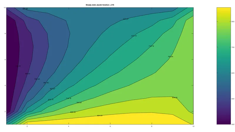
figure(1)
contourf(flipud(T),'Showtext','ON')
title(sprintf('Steady state Jacobi iteration = %d',jac_iter))
pause(0.005)
colorbar
end


%reinitializing
T = T_initial
Told = T
error = 9e9

% Gauss Seidel

gs_iter = 0
while(error > tol)

for i = 2:nx-1
  for j = 2:ny-1

    T(i,j) = 0.25*(Told(i+1,j) + T(i-1,j) + T(i,j-1) + Told(i,j+1))
  end
end

error = max(max(abs(T-Told)))

Told = T
gs_iter = gs_iter + 1
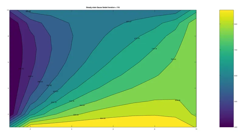
figure(2)
contourf(flipud(T),'Showtext','ON')
title(sprintf('Steady state Gauss Seidel iteration = %d',gs_iter))
pause(0.005)
colorbar
end


%reinitializing
T = T_initial
Told = T
error = 9e9

%Successive Over Relaxation

sor_iter = 0
omega = 1.5
while(error > tol)

for i = 2:nx-1
  for j = 2:ny-1

    TGS(i,j) = 0.25*(Told(i+1,j) + T(i-1,j) + T(i,j-1) + Told(i,j+1))
    T(i,j) = (1-omega)*Told(i,j) + omega*TGS(i,j)
  end
end

error = max(max(abs(T-Told)))

Told = T
sor_iter = sor_iter + 1
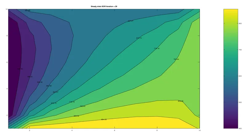
figure(3)
contourf(flipud(T),'Showtext','ON')
title(sprintf('Steady state SOR iteration = %d',sor_iter))
pause(0.005)
colorbar
end
Output
1.Jacobi
2.Gauss Seidel
3.Successive over Relaxation (SOR)
Transient implicit code
close all
clear all
clc

% steady state heat conduction equation d^2T/dx^2 + d^2T/dy^2 = 0

nx = 10
ny = 10

T = ones(nx,ny)

% temperatures
TL = 400
TR = 800
TT = 600
TB = 900

% Boundary conditions
T(:,1) = TL
T(:,ny) = TR
T(1,:) = TT
T(nx,:) = TB

% Edge refinement
T(1,1) = 0.5*(T(2,1) + T(1,2))
T(nx,1) = 0.5*(T(nx-1,1) + T(nx,2))
T(nx,ny) = 0.5*(T(nx-1,ny) + T(nx,ny-1))
T(1,ny) = 0.5*(T(2,ny) + T(1,ny-1))


Told = T
T_initial = T
Tprev = T

%time step
dt = 1e-2

% grid spacing
dx = 1e-2
dy = 1e-2


% Thermal diffusivity
alpha = 0.015


k1 = alpha*dt/dx^2
k2 = alpha*dt/dy^2

% iterative solver =
% Jacobi

error = 9e9
conv = 9e9
tol = 1e-4

jac_iter = 0
jac_time_iter = 0

% time loop
while(conv > tol)
% space loop
while(error > tol)

for i = 2:nx-1
  for j = 2:ny-1

    T(i,j) = (1+2*k1+2*k2)^-1*(Tprev(i,j) + k1*(Told(i-1,j) + Told(i+1,j)) + k2*(Told(i,j-1) + Told(i,j+1)))
   end
end

error = max(max(abs(T-Told)))

Told = T
jac_iter = jac_iter + 1
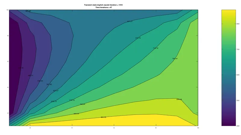
figure(1)
contourf(flipud(T),'Showtext','ON')
title(sprintf('Transient state implicit Jacobi iteration = %d \n Time iterations = %d',jac_iter,jac_time_iter))
pause(0.005)
colorbar
end
conv = max(max(abs(T-Tprev)))
Tprev = T
jac_time_iter = jac_time_iter + 1
error = 9e9
end


%reinitializing
T = T_initial
Told = T
Tprev = T
error = 9e9
conv = 9e9

% Gauss Seidel

gs_iter = 0
gs_time_iter = 0
% time loop
while(conv > tol)
% space loop
while(error > tol)

for i = 2:nx-1
  for j = 2:ny-1

    T(i,j) = (1+2*k1+2*k2)^-1*(Tprev(i,j) + k1*(T(i-1,j) + Told(i+1,j)) + k2*(T(i,j-1) + Told(i,j+1)))
   end
end

error = max(max(abs(T-Told)))

Told = T
gs_iter = gs_iter + 1
figure(2)
contourf(flipud(T),'Showtext','ON')
title(sprintf('Transient state implicit GS iteration = %d \n Time iterations = %d',gs_iter,gs_time_iter))
pause(0.005)
colorbar
end
conv = max(max(abs(T-Tprev)))
Tprev = T
gs_time_iter = gs_time_iter + 1
error = 9e9
end


%reinitializing
T = T_initial
Told = T
Tprev = T
error = 9e9
conv = 9e9


%Successive Over Relaxation

sor_iter = 0
sor_time_iter = 0
omega = 1.5
% time loop
while(conv > tol)
% space loop
while(error > tol)

for i = 2:nx-1
  for j = 2:ny-1

    TGS(i,j) = (1+2*k1+2*k2)^-1*(Tprev(i,j) + k1*(T(i-1,j) + Told(i+1,j)) + k2*(T(i,j-1) + Told(i,j+1)))
    T(i,j) = (1-omega)*Told(i,j) + omega*(TGS(i,j))
   end
end

error = max(max(abs(T-Told)))

Told = T
sor_iter = sor_iter + 1
figure(3)
contourf(flipud(T),'Showtext','ON')
title(sprintf('Transient state implicit SOR iteration = %d \n Time iterations = %d',sor_iter,sor_time_iter))
pause(0.005)
colorbar
end
conv = max(max(abs(T-Tprev)))
Tprev = T
sor_time_iter = sor_time_iter + 1
error = 9e9
end
Jacobi
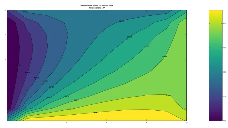
Gauss Seidel
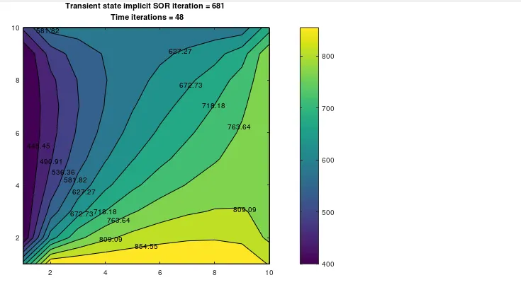
SOR
Transient Explicit code
close all
clear all
clc

% steady state heat conduction equation d^2T/dx^2 + d^2T/dy^2 = 0

nx = 10
ny = 10

T = ones(nx,ny)

% temperatures
TL = 400
TR = 800
TT = 600
TB = 900

% Boundary conditions
T(:,1) = TL
T(:,ny) = TR
T(1,:) = TT
T(nx,:) = TB

% Edge refinement
T(1,1) = 0.5*(T(2,1) + T(1,2))
T(nx,1) = 0.5*(T(nx-1,1) + T(nx,2))
T(nx,ny) = 0.5*(T(nx-1,ny) + T(nx,ny-1))
T(1,ny) = 0.5*(T(2,ny) + T(1,ny-1))


Tprev = T

%time step
dt = 1e-2

% grid spacing
dx = 5e-2
dy = 5e-2


% Thermal diffusivity
alpha = 0.015


k1 = alpha*dt/dx^2
k2 = alpha*dt/dy^2

cfl = k1+k2

conv = 9e9
tol = 1e-4

time_iter = 0

% time loop
while(conv > tol)
for i = 2:nx-1
  for j = 2:ny-1

    T(i,j) = (1-2*k1-2*k2)*Tprev(i,j) + k1*(Tprev(i-1,j) + Tprev(i+1,j)) + k2*(Tprev(i,j-1) + Tprev(i,j+1))
   end
end

conv = max(max(abs(T-Tprev)))
Tprev = T
time_iter = time_iter + 1
figure(1)
contourf(flipud(T),'Showtext','ON')
title(sprintf('Transient state explicit iteration = %d',time_iter))
pause(0.005)
colorbar
end
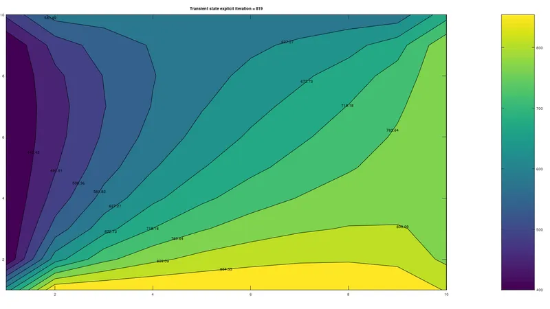
Transient explicit diagram
Results and Conclusions
From the above graphs we can say that
1.When we compare steadyc and unsteady state , steady state is the most successful as it takes least number of iterations and least time to compute.
2.SOR iteration is the most effective amongst the 3 as it took less number of iterations from both the ways.
3.For transient equations time required to solve is more compared to steady state equations.So, therefore it is recommended to solve the 2D heat conduction equation with steady state conditions.