Week 7 - Simulation of a 1D Super-sonic nozzle flow simulation using Macormack Method
Objective;
To stimulate the isentropic flow through a quasi id subsonic-supersonic nozzle by deriving both the conservative and non-conservative forms of the governing equations and solve them using MacCarmack technique by determining the steady-state temperature distribution for the flow field variable and investigate the difference between the 2 forms of governing equation by comparing the solution stated below;
1.Steady-state distribution of primitive variables inside the nozzle.
2.Time-wise variation of the primitive variable.
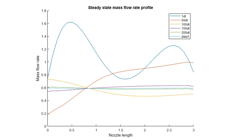
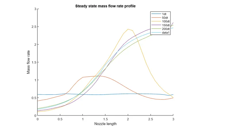
3.Variation of mass flow rate distribution inside the nozzle at different time steps during time-marching process.
Theory
Any numerical solution of isentropic flow through quasi 1d subsonic-supersonic nozzle is unreasonable,while analytic solution exists for these kind of problems. Here, we are establishing the broadened capability of CFD in various streams rather than representing the form of analytic solution.In this challenge we implement the numerical solution with conservative and non-conservative forms.
Macormack Method
1.To discretize the numerical solution we use the technique called MacCarmack method.This method is a variation of the 2 step Lax-Wendroff scheme but is much simpler in application.
2.It is also the explicit finite difference technique which is second order accurate in both time and space.
3.This method is very effective where we can obtain second order accuracy with first order terms and mathematical complexity of calculating the second order time derivative can be avoided.
Non-conservative form
clear all
close all
clc

% inputs
n = 31;
x = linspace(0,3,n);
dx = x(2)-x(1);
gamma = 1.4;

% calculate initial profiles
rho = 1-0.3146*x;
t = 1-0.2314*x; % t = temperature
v = (0.1+1.09*x).*t.^0.5;

a = 1+2.2*(x-1.5).^2;

% time steps
nt = 1400;
dt = 0.04;

th = round(n/2)

cfl = max((v + sqrt(t))*dt/dx)

% outer time loop
for k = 1:nt

    rho_old = rho;
    v_old = v;
    t_old = t;


    %predictor method
    for j = 2:n-1
        %drho_dt_p = -rho(j)*(v(j+1)-v(j))/dx -rho(j)*v(j)*(log(a(j+1))-log(a(j)))/dx -v(j)*(rho(j+1)-rho(j))/dx
        dvdx = (v(j+1)-v(j))/dx;
        drhodx = (rho(j+1)-rho(j))/dx;
        dtdx = (t(j+1)-t(j))/dx;
        dlogadx = (log(a(j+1))-log(a(j)))/dx;

        % continuity equation
        drhodt_p(j) = -rho(j)*dvdx -rho(j)*v(j)*dlogadx -v(j)*drhodx;
        % momentum equation
        dvdt_p(j) = -v(j)*dvdx -(1/gamma)*(dtdx + (t(j)/rho(j))*drhodx);
        % energy
        dtdt_p(j) = -v(j)*dtdx - (gamma-1)*t(j)*(dvdx + v(j)*dlogadx);

         % solution update
         rho(j) = rho(j) + drhodt_p(j)*dt;
         v(j) = v(j) + dvdt_p(j)*dt;
         t(j) = t(j) + dtdt_p(j)*dt;
    end

    % corrector method
    for j = 2:n-1
        %drho_dt_p = -rho(j)*(v(j+1)-v(j))/dx -rho(j)*v(j)*(log(a(j+1))-log(a(j)))/dx -v(j)*(rho(j+1)-rho(j))/dx
        dvdx = (v(j)-v(j-1))/dx;
        drhodx = (rho(j)-rho(j-1))/dx;
        dtdx = (t(j)-t(j-1))/dx;
        dlogadx = (log(a(j))-log(a(j-1)))/dx;

        % continuity equation
        drhodt_c(j) = -rho(j)*dvdx -rho(j)*v(j)*dlogadx -v(j)*drhodx;
        % momentum equation
        dvdt_c(j) = -v(j)*dvdx -(1/gamma)*(dtdx + (t(j)/rho(j))*drhodx);
        % energy
        dtdt_c(j) = -v(j)*dtdx - (gamma-1)*t(j)*(dvdx + v(j)*dlogadx);

    end
   % compute the average time derivative

   drhodt = 0.5*(drhodt_p + drhodt_c)
   dvdt = 0.5*(dvdt_p + dvdt_c)
   dtdt = 0.5*(dtdt_p + dtdt_c)

   % Final solution update
   for i = 2:n-1
       rho(i) = rho_old(i) + drhodt(i)*dt
       v(i) = v_old(i) + dvdt(i)*dt
       t(i) = t_old(i) + dtdt(i)*dt
   end
   % Boundary conditions
   % At inlet
   v(1) = 2*v(2) - v(3)
   % At outlet
   v(n) = 2*v(n-1) - v(n-2)
   rho(n) = 2*rho(n-1) - rho(n-2)
   t(n) = 2*t(n-1) - t(n-2)

   % Pressure
   p = rho.*t
   % Mach Number
   M = v./sqrt(t)
   % Mass Flow rate
   m = rho.*a.*v
figure(3)
hold on
if k == 1
    plot(x,m)
end
if k == 50
    plot(x,m)
end
if k == 100
    plot(x,m)
end
if k == 150
    plot(x,m)
end
if k == 200
    plot(x,m)
end

rho_throat(k) = rho(th)
v_throat(k) = v(th)
t_throat(k) = t(th)
p_throat(k) = p(th)
M_throat(k) = M(th)


end

xlabel('Nozzle length')
ylabel('Mass flow rate')
legend('1dt','50dt','100dt','150dt','200dt')
title('Variation of mass flow rate at different time steps')

figure(1)
subplot(5,1,1)
plot(x,v)
xlabel('Nozzle length')
ylabel('Velocity')
title('Transient varation of primitive variable profiles at throat')
subplot(5,1,2)
plot(x,rho)
xlabel('Nozzle length')
ylabel('Density')
subplot(5,1,3)
plot(x,t)
xlabel('Nozzle length')
ylabel('Temperature')
subplot(5,1,4)
plot(x,p)
xlabel('Nozzle length')
ylabel('Pressure')
subplot(5,1,5)
plot(x,M)
xlabel('Nozzle length')
ylabel('Mack number')

figure(2)
subplot(5,1,1)
plot(v_throat)
xlabel('Time step')
ylabel('Velocity')
title('Transient varation of primitive variable profiles at throat')
subplot(5,1,2)
plot(rho_throat)
xlabel('Time step')
ylabel('Density')
subplot(5,1,3)
plot(t_throat)
xlabel('Time step')
ylabel('Temperature')
subplot(5,1,4)
plot(p_throat)
xlabel('Time step')
ylabel('Pressure')
subplot(5,1,5)
plot(M_throat)
xlabel('Time step')
ylabel('Mack number')

figure(3)
plot(x,m)
title('Steady state mass flow rate profile')
xlabel('Nozzle length')
ylabel('Mass flow rate')
Conservative form
clear all
close all
clc
% inputs
n = 31;
x = linspace(0,3,n);
dx = x(2)-x(1);
gamma = 1.4;
% calculate initial profiles
%rho = 1-0.3146*x;
%t = 1-0.2314*x; % t = temperature
%v = (0.1+1.09*x).*t.^0.5;
for i = 1:n
    if x(i) <= 0.5
        rho(i) = 1
        t(i) = 1
    end

    if x(i) > 0.5 && x(i) <= 1.5
        rho(i) = 1-0.366*(x(i)-0.5)
        t(i) = 1-0.167*(x(i)-0.5)
    end
     if x(i) > 1.5
        rho(i) = 0.634 - 0.3879*(x(i)-1.5)
        t(i) = 0.833-0.3507*(x(i)-1.5)
    end
end

nt = 1400;
dt = 0.0267;
th = round(n/2)

a = 1+2.2*(x-1.5).^2;

v = 0.59./(rho.*a)

U1 = rho.*a
U2 = rho.*a.*v
U3 = U1.*(t/(gamma-1) + (gamma/2)*v.^2)


cfl = max((v + sqrt(t))*dt/dx)
% outer time loop
for k = 1:nt

    U1_old = U1;
    U2_old = U2;
    U3_old = U3;

    F1 = U1
    F2 = U2.^2./U1 + ((gamma-1)/gamma)*(U3 - (gamma/2)*(U2.^2./U1))
    F3 = gamma*U2.*U3./U1 - 0.5*gamma*(gamma-1)

    %predictor method
    for j = 2:n-1

       % continuity equation
        dU1dt_p(j) = -(F1(j+1)-F1(j))/dx

        J2 = (1/gamma)*rho(j)*t(j)*(a(j+1)-a(j))/dx;

       % momentum equation
        dU2dt_p(j) = -(F2(j+1)-F2(j))/dx + J2

        % energy
        dU3dt_p(j) = -(F3(j+1)-F3(j))/dx

        % solution update
         U1(j) = U1(j) + dU1dt_p(j)*dt;
         U2(j) = U2(j) + dU2dt_p(j)*dt;
         U3(j) = U3(j) + dU3dt_p(j)*dt;
    end

    % Predictor update
    rho = U1./a;
    t = (gamma-1)*(U3./U1 - (gamma/2)*(U2./U1).^2)
    F1 = U1
    F2 = U2.^2./U1 + ((gamma-1)/gamma)*(U3 - (gamma/2)*(U2.^2./U1))
    F3 = gamma*U2.*U3./U1 - 0.5*gamma*(gamma-1)

    % corrector method
    for j = 2:n-1


        % continuity equation
        dU1dt_c(j) = -(F1(j)-F1(j-1))/dx

        J2 = (1/gamma)*rho(j)*t(j)*(a(j)-a(j-1))/dx;

       % momentum equation
        dU2dt_c(j) = -(F2(j)-F2(j-1))/dx + J2

        % energy
        dU3dt_c(j) = -(F3(j)-F3(j-1))/dx
    end

    % compute the average time derivative
   dU1dt = 0.5*(dU1dt_p + dU1dt_c)
   dU2dt = 0.5*(dU2dt_p + dU2dt_c)
   dU3dt = 0.5*(dU3dt_p + dU3dt_c)
   % Final solution update
   for i = 2:n-1
       U1(i) = U1_old(i) + dU1dt(i)*dt
       U2(i) = U2_old(i) + dU2dt(i)*dt
       U3(i) = U3_old(i) + dU3dt(i)*dt
   end

   % Corrector update
   rho = U1./a;
   t = (gamma-1)*(U3./U1 - (gamma/2)*(U2./U1).^2)
   v = U2./U1

   % Boundary conditions
   % At inlet
   U1(1) = a(1)
   U2(1) = 2*U2(2) - U2(3)
   U3(1) = U1(1)*(t(1)/(gamma-1) + 0.5*gamma*v(1)^2)
   % At outlet
   U1(n) = 2*U1(n-1) - U1(n-2)
   U2(n) = 2*U2(n-1) - U2(n-2)
   U3(n) = 2*U3(n-1) - U3(n-2)


   % Pressure
   p = rho.*t
   % Mach Number
   M = v./sqrt(t)
   % Mass Flow rate
   m = rho.*a.*v

   figure(3)
hold on
if k == 1
    plot(x,m)
end
if k == 50
    plot(x,m)
end
if k == 100
    plot(x,m)
end
if k == 150
    plot(x,m)
end
if k == 200
    plot(x,m)
end
rho_throat(k) = rho(th)
v_throat(k) = v(th)
t_throat(k) = t(th)
p_throat(k) = p(th)
M_throat(k) = M(th)

end
xlabel('Nozzle length')
ylabel('Mass flow rate')
legend('1dt','50dt','100dt','150dt','200dt')
title('Variation of mass flow rate at different time steps')
figure(1)
subplot(5,1,1)
plot(x,v)
xlabel('Nozzle length')
ylabel('Velocity')
title('Transient varation of primitive variable profiles at throat')
subplot(5,1,2)
plot(x,rho)
xlabel('Nozzle length')
ylabel('Density')
subplot(5,1,3)
plot(x,t)
xlabel('Nozzle length')
ylabel('Temperature')
subplot(5,1,4)
plot(x,p)
xlabel('Nozzle length')
ylabel('Pressure')
subplot(5,1,5)
plot(x,M)
xlabel('Nozzle length')
ylabel('Mack number')
figure(2)
subplot(5,1,1)
plot(v_throat)
xlabel('Time step')
ylabel('Velocity')
title('Transient varation of primitive variable profiles at throat')
subplot(5,1,2)
plot(rho_throat)
xlabel('Time step')
ylabel('Density')
subplot(5,1,3)
plot(t_throat)
xlabel('Time step')
ylabel('Temperature')
subplot(5,1,4)
plot(p_throat)
xlabel('Time step')
ylabel('Pressure')
subplot(5,1,5)
plot(M_throat)
xlabel('Time step')
ylabel('Mack number')
figure(3)
plot(x,m)
title('Steady state mass flow rate profile')
xlabel('Nozzle length')
ylabel('Mass flow rate')
The corresponding graphs are formed
Figure 1
Non conservative form
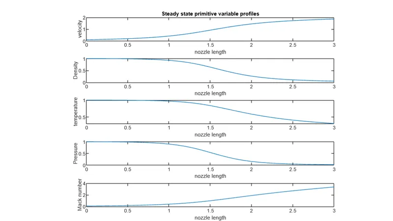
Figure 2
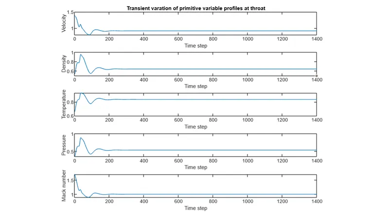
Figure 3
Conservative form
Figure 1
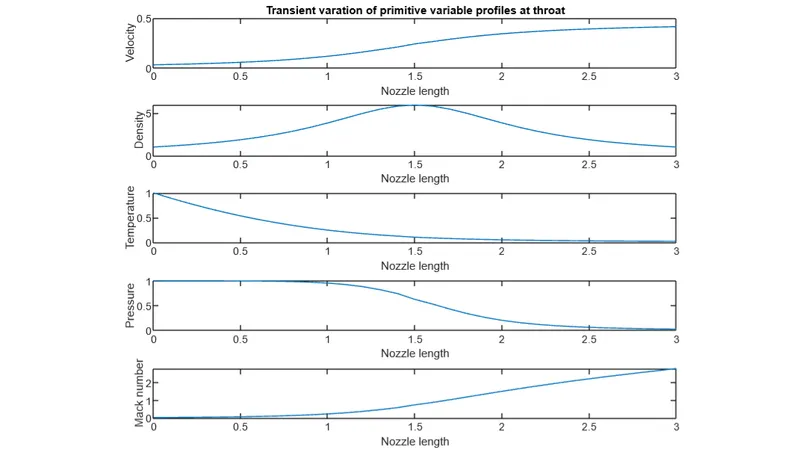
Figure 2
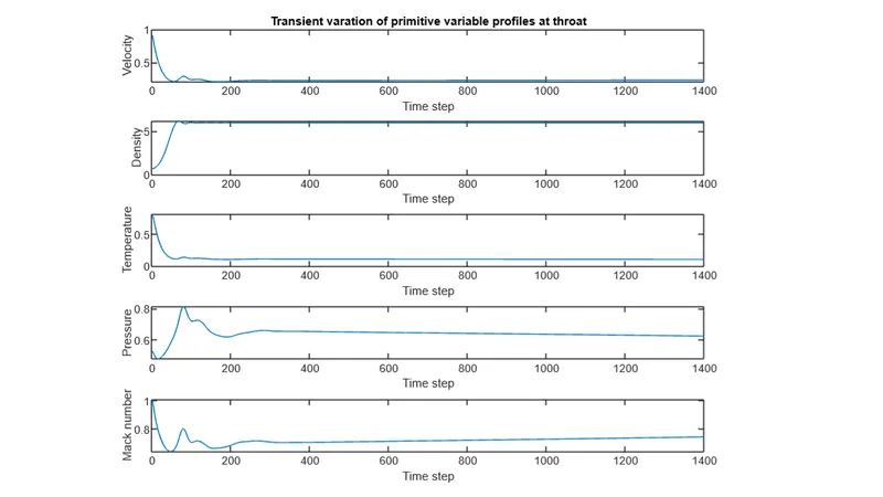
Figure 3
Conclusion
1.In the steady state graph we can see that both are in same phase giving the same exact solution.
2.In the transient state graph we can conclude that initial variations observed in non-conservative form for a certain period of time makes it consume higher amount of time to achieve stable solution compared to conservative form.
3.In the mass flow rate plot is shows that at different time steps along distance oscillates initially, however the solution becomes stable after the 400th time step for both forms attaining a constant value.
4.Finally, we can conclude that, conservative form converges slightly faster than non conservative form offering stable solution .Yet both the forms are dependable in calculating the solution which is almost precise.