Week 11 - Simulation of Flow through a pipe in OpenFoam
Incompressible laminar flow through a pipe:
Hagen-Poiseuille's equation provides analytical solution for pressure drop due to fluid viscosity in a pipe of constant cross-section having incompressible laminar flow. The goal of this exercise is to simulate Hagen-Poiseuille's flow with axisymmetric approximation in OpenFoam and compare the results with analytical solution. Reynolds number, `Re` of the flow is given to be 2100. We assume, the diameter of the pipe, `D` to be 0.01 [m]. Flowing medium is assumed to be water. Hence density of fluid, `rho` is 1000 [kg/m^3] and dynamic viscosity, `mu` will be 1e-3 [Pa s]. Boundary layers formed along the wall of pipe due to viscosity of the fluid will grow along the pipe and coincide at the axis of pipe after a certain length. Beyond this point, the velocity profile and wall shear stress becomes constant. The length of pipe required to achive this constant wall shear stress is termed as hydrodynamic entry length.
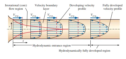
Courtesy: Fluid Mechanics, Yunus A.Cengel
Entry length is approximated using following formula for laminar flows.
`L_h ~= 0.05 * Re * D = 0.05 * 2100 * 0.01 = 1.05 [m]`
The effect of entry region will increase the pressure drop of fluid greater than the value approximated by Hagen-Poiseuille's equation. To reduce the effect of entrance region to negligible values, the length of pipe must be much larger than the entrance lenth. Hence, to reduce the effect of entrance length and also keep the computational cost at a reasoble level, the length of pipe, `L` is assumed to be 11.55 [m], an order of magnitude greater than the entrance length.
The velocity profile for fully developed laminar flow in pipe will have a parabolic shape with zero velocity at walls and max velocity occurring at the axis. After this point, the velocity gradient along the flow direction will become zero. Velocity can be described as a function of radius of pipe only.
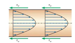
Courtesy: Fluid Mechanics, Yunus A.Cengel
Velocity as a function of radius is given by following expression.
`V(r) = 2V_(avg)(1-r^2/R^2)` -------------- (1)
where, `V_(avg)` -> average velocity of flow in pipe
`r` -> local radius of pipe
`R` -> max radius of pipe
Maximum velocity at the axis of pipe is given by
`V_(max) = 2* V_(avg)` -------------- (2)
Hagen-Poiseuille's equation of pressure drop for a full developed laminar flow in a pipe is given by
`Deltap = (32muLV_(avg))/D^2` ---------------- (3)
where, `mu` -> viscosity of fluid
`L` -> length of pipe
So, the input parameters for the problem are given by,
`Re` = 2100
`D` = 0.01 [m]
`L` = 11.55 [m]
`rho` = 1000 [kg/m^3]
`mu` = 1e-3 [Pa s]
Velocity at inlet can be calculated from `Re` using
`V_("inlet") = (Re*mu)/(rhoD) = (2100*10^-3)/ (1000 * 0.01) = 0.21 [m//s]`
Simulation of Hagen-Poiseuille's flow using OpenFoam:
Since the flow has an axisymmetric nature, the simulation is carried on a small sector of the pipe using wedge boundary condition. This will solve the problem in 2D using axisymmetric assumption. The wedge faces are placed on either side of xy plane with wedge half angle of 1 degree. The angle of this wedge doesn't have much of an importance, since the domain is solved in 2D. However the wedge angle should be less than 5 degress for axisymmetric domains used in openFoam solver.
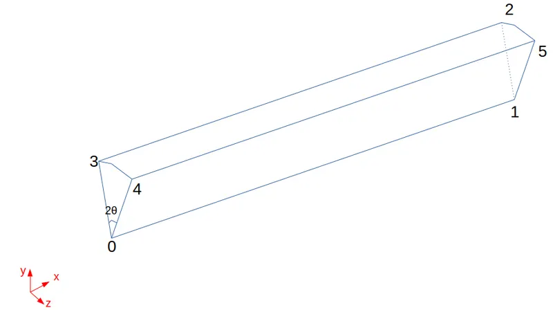
Number cells across the wedge faces is 1. Number of faces across the radial direction is taken to be 20. Cell size grading along radial direction is chosen to be constant, since velocity gradient is significant over all values of `r` after the entry length. To maintain the aspect ratio of cells below 100, the number of cells in x direction is chosen to 500.
1. Generating blockMeshDict file using Matlab
A matlab progam is written that takes the input variables such as domain extents, number cells, etc and creates a blockMeshDict file based on a sample Dict file.
% Create blockMeshDict file to generate a wedge to simulate axisymmetric flow
% through pipe from a sample Dict file
clear all
close all
clc

% sample and target file locations
baseFile = 'blockMeshDict_sample';
targetFile = 'blockMeshDict';

% wedge details
scalingFactor = 1;        % scale factor to meters
length = 11.55;           % length of cylinder
dia = 0.01;               % diameter of pipe
wedgeAngle = 2;           % wedge angle

% number of cells
nx = 500;           % along length of cylinder
ny = 20;            % along radial direction
gd = 1;           % grading factor from axis to wall of cylinder

% calculate required parameters
radius = dia/2;             % radius of pipe
theta = wedgeAngle/2;       % wedge half angle

% open base and target files
bfp = fopen(baseFile,'r');
tfp = fopen(targetFile,'w');

%Copy header info from base file
bfd = fgets(bfp);   % read first line
while ~contains(bfd,"convertToMeters")
    fprintf(tfp, '%s\n', bfd);
    bfd = fgetl(bfp);
    if bfd == -1
        disp('Error: Sample file incorrect!')
        fclose(tfp);
        break
    end
end

% close base file
fclose(bfp);

% calculate vertices
v = zeros(6,3);            % 6 points are used to define a wedge
v(1,:) = [0 0 0];
v(2,:) = [length 0 0];
v(3,:) = [length radius*cosd(theta) -radius*sind(theta)];
v(4,:) = [0 radius*cosd(theta) -radius*sind(theta)];
v(5,:) = [0 radius*cosd(theta) radius*sind(theta)];
v(6,:) = [length radius*cosd(theta) radius*sind(theta)];

% print vertices to target file
fprintf(tfp,'vertices\n(\n');
for i = 1:size(v,1)
    fprintf(tfp,'\t(%g %g %g)\n',v(i,:));
end
fprintf(tfp,');\n\n');

% calculate interpolation points for arc
ips = zeros(2,3);
ips(1,:) = [0 radius 0];
ips(2,:) = [length radius 0];

% print edges to target file
fprintf(tfp,'edges\n(\n');
fprintf(tfp,'\tarc 3 4(%g %g %g)\n',ips(1,:));
fprintf(tfp,'\tarc 2 5(%g %g %g)\n',ips(2,:));
fprintf(tfp,');\n\n');

% define and print blocks to target file
fprintf(tfp,'blocks\n(\n');
fprintf(tfp,'\thex (0 1 2 3 0 1 5 4) (%d %d 1) simpleGrading (1 %f 1)\n',nx,ny,gd);
fprintf(tfp,');\n\n');

% define boundaries
axis = [0 1 1 0];
inlet = [0 4 3 0];
outlet = [1 2 5 1];
top = [3 4 5 2];
front= [0 1 5 4];
back = [0 3 2 1];

% Print boundaries to target file
fprintf(tfp,'boundary\n(\n');
%axis
fprintf(tfp,'\taxis\n\t{\n\t\ttype empty;\n\t\tfaces\n\t\t(\n\t\t\t(%d %d %d %d)\n\t\t);\n\t}\n',axis);
%inlet
fprintf(tfp,'\tinlet\n\t{\n\t\ttype patch;\n\t\tfaces\n\t\t(\n\t\t\t(%d %d %d %d)\n\t\t);\n\t}\n',inlet);
%outlet
fprintf(tfp,'\toutlet\n\t{\n\t\ttype patch;\n\t\tfaces\n\t\t(\n\t\t\t(%d %d %d %d)\n\t\t);\n\t}\n',outlet);
%wall
fprintf(tfp,'\twall\n\t{\n\t\ttype wall;\n\t\tfaces\n\t\t(\n\t\t\t(%d %d %d %d)\n\t\t);\n\t}\n',top);
%front
fprintf(tfp,'\tfront\n\t{\n\t\ttype wedge;\n\t\tfaces\n\t\t(\n\t\t\t(%d %d %d %d)\n\t\t);\n\t}\n',front);
%back
fprintf(tfp,'\tback\n\t{\n\t\ttype wedge;\n\t\tfaces\n\t\t(\n\t\t\t(%d %d %d %d)\n\t\t);\n\t}\n',back);
fprintf(tfp,');\n\n');

% close target file
fprintf(tfp,'// %s //\n',repmat('*',80,1));
fclose(tfp);
disp('Success: blockMeshDict created')
The output blockMeshDict is as shown below. A sample blockMeshDict is used from one of the tutorials to copy the generic data to new file.
/*--------------------------------*- C++ -*----------------------------------*\

  =========                 |
  \\      /  F ield         | OpenFOAM: The Open Source CFD Toolbox
   \\    /   O peration     | Website:  https://openfoam.org
    \\  /    A nd           | Version:  9
     \\/     M anipulation  |
\*---------------------------------------------------------------------------*/
FoamFile
{
    format      ascii;
    class       dictionary;
    object      blockMeshDict;
}
// * * * * * * * * * * * * * * * * * * * * * * * * * * * * * * * * * * * * * //

// Note: this file is a Copy of $FOAM_TUTORIALS/resources/blockMesh/pitzDaily

vertices
(
	(0 0 0)
	(11.55 0 0)
	(11.55 0.00499924 -8.7262e-05)
	(0 0.00499924 -8.7262e-05)
	(0 0.00499924 8.7262e-05)
	(11.55 0.00499924 8.7262e-05)
);

edges
(
	arc 3 4(0 0.005 0)
	arc 2 5(11.55 0.005 0)
);

blocks
(
	hex (0 1 2 3 0 1 5 4) (500 20 1) simpleGrading (1 1.000000 1)
);

boundary
(
	axis
	{
		type empty;
		faces
		(
			(0 1 1 0)
		);
	}
	inlet
	{
		type patch;
		faces
		(
			(0 4 3 0)
		);
	}
	outlet
	{
		type patch;
		faces
		(
			(1 2 5 1)
		);
	}
	wall
	{
		type wall;
		faces
		(
			(3 4 5 2)
		);
	}
	front
	{
		type wedge;
		faces
		(
			(0 1 5 4)
		);
	}
	back
	{
		type wedge;
		faces
		(
			(0 3 2 1)
		);
	}
);

// ******************************************************************************** //
2. Inital conditions, boundary conditions and solver settings
Since the problem is incompressible laminar flow, icoFoam solver is best suited for this simulation. Hence, the elbow tutorial for icoFoam solver is copied to foam run directory and renamed to pipe. The mesh file in the tutorial is removed and the blockMeshDict file generated previously is placed inside the system folder. "blockMesh" command is called inside the pipe folder. Mesh file is generated. Next step is to setup the boundary and initial condition inside the "0" folder of the test. IcoFoam solves for a scalar-> kinematic pressure and vector-> velocity through the domain on each cell centroid. Since density is constant for incompressible flow, kinematic pressure which represents the ratio of gauge pressure to density is used to reduce the number of parameters in the solution process. For incompressible flow, the best choice of boundary conditions -> velocity inlet and presure outlet, is used to define the problem. Gauge pressure at outlet is zero. Hence, kinematic pressure is also 0. Velocity at inlet is 0.21 [m/s] in x-direction as calculated above. The domain is initialized to 0 kinematic pressure at 0th time-step. Velocity in the domain is initialized to 0.21 [m/s] in x-direction, same as that of inlet, so steady state can be achieved in less number of time-steps. Hence, the boundary/initial definition files in 0 folder are set as follows
/*--------------------------------*- C++ -*----------------------------------*\
  =========                 |
  \\      /  F ield         | OpenFOAM: The Open Source CFD Toolbox
   \\    /   O peration     | Website:  https://openfoam.org
    \\  /    A nd           | Version:  9
     \\/     M anipulation  |
\*---------------------------------------------------------------------------*/
FoamFile
{
    format      ascii;
    class       volScalarField;
    object      p;
}
// * * * * * * * * * * * * * * * * * * * * * * * * * * * * * * * * * * * * * //

dimensions      [0 2 -2 0 0 0 0];

internalField   uniform 0;

boundaryField
{
    inlet
    {
        type            zeroGradient;
    }

    wall
    {
        type            zeroGradient;
    }

    outlet
    {
        type            fixedValue;
        value           uniform 0;
    }

    axis
    {
        type            empty;
    }

    front
    {
        type            wedge;
    }

    back
    {
        type            wedge;
    }
}

// ************************************************************************* //
/*--------------------------------*- C++ -*----------------------------------*\
  =========                 |
  \\      /  F ield         | OpenFOAM: The Open Source CFD Toolbox
   \\    /   O peration     | Website:  https://openfoam.org
    \\  /    A nd           | Version:  9
     \\/     M anipulation  |
\*---------------------------------------------------------------------------*/
FoamFile
{
    format      ascii;
    class       volVectorField;
    object      U;
}
// * * * * * * * * * * * * * * * * * * * * * * * * * * * * * * * * * * * * * //

dimensions      [0 1 -1 0 0 0 0];

internalField   uniform (0.21 0 0);

boundaryField
{
    inlet
    {
        type            fixedValue;
        value           uniform (0.21 0 0);
    }

    outlet
    {
        type            zeroGradient;
    }

    axis
    {
        type            empty;
    }

    wall
    {
        type            noSlip;
    }

    front
    {
        type            wedge;
    }

    back
    {
        type            wedge;
    }
}

// ************************************************************************* //
The constant property, kinematic viscosity is to be provided in "transportProperties" file in constant folder
kinematic viscosity, `nu = mu/rho = 10^-3/1000 = 10^-6`
/*--------------------------------*- C++ -*----------------------------------*\
  =========                 |
  \\      /  F ield         | OpenFOAM: The Open Source CFD Toolbox
   \\    /   O peration     | Website:  https://openfoam.org
    \\  /    A nd           | Version:  9
     \\/     M anipulation  |
\*---------------------------------------------------------------------------*/
FoamFile
{
    format      ascii;
    class       dictionary;
    location    "constant";
    object      transportProperties;
}
// * * * * * * * * * * * * * * * * * * * * * * * * * * * * * * * * * * * * * //

nu              [0 2 -1 0 0 0 0] 0.000001;


// ************************************************************************* //
The solution controls and schemes are set in files under system folder. With cell length in x-direction, `dx = 11.55/500 = 0.0231`. For an initial trial, an average value of 1 is chosen for CFL number. Hence, time-step size can be calculated using, `dt = (CFL * dx)/V_x = (1*0.0231)/0.21 ~= 0.1`. This time-step is used in the solution and solution is solved for 100 [s] of simulation time. This simulation time represents approximately 2 complete flow-through time of fluid from inlet to outlet, `t = L / V = 11.55 /0.21 = 55 [s]`. With provided good initial guess, the solution would attain steady state within this stipulated time. In "fvSchemes" file under system folder, divergence scheme-> "div(phi,U)" is updated from "Gauss limitedLinearV 1" to simple "Gauss linear" method. This scheme is much suited for structured mesh used in this simulation and increase the convergence speed. Solver setttings in "fvSolution" file in not modified. The solution control files as shown below.
/*--------------------------------*- C++ -*----------------------------------*\
  =========                 |
  \\      /  F ield         | OpenFOAM: The Open Source CFD Toolbox
   \\    /   O peration     | Website:  https://openfoam.org
    \\  /    A nd           | Version:  9
     \\/     M anipulation  |
\*---------------------------------------------------------------------------*/
FoamFile
{
    format      ascii;
    class       dictionary;
    location    "system";
    object      controlDict;
}
// * * * * * * * * * * * * * * * * * * * * * * * * * * * * * * * * * * * * * //

application     icoFoam;

startFrom       latestTime;

startTime       0;

stopAt          endTime;

endTime         100;

deltaT          0.1;

writeControl    timeStep;

writeInterval   100;

purgeWrite      0;

writeFormat     ascii;

writePrecision  6;

writeCompression off;

timeFormat      general;

timePrecision   6;

runTimeModifiable true;


// ************************************************************************* //
/*--------------------------------*- C++ -*----------------------------------*\
  =========                 |
  \\      /  F ield         | OpenFOAM: The Open Source CFD Toolbox
   \\    /   O peration     | Website:  https://openfoam.org
    \\  /    A nd           | Version:  9
     \\/     M anipulation  |
\*---------------------------------------------------------------------------*/
FoamFile
{
    format      ascii;
    class       dictionary;
    location    "system";
    object      fvSchemes;
}
// * * * * * * * * * * * * * * * * * * * * * * * * * * * * * * * * * * * * * //

ddtSchemes
{
    default         Euler;
}

gradSchemes
{
    default         Gauss linear;
}

divSchemes
{
    default         none;
    div(phi,U)      Gauss linear;
}

laplacianSchemes
{
    default         Gauss linear corrected;
}

interpolationSchemes
{
    default         linear;
}

snGradSchemes
{
    default         corrected;
}


// ************************************************************************* //
/*--------------------------------*- C++ -*----------------------------------*\
  =========                 |
  \\      /  F ield         | OpenFOAM: The Open Source CFD Toolbox
   \\    /   O peration     | Website:  https://openfoam.org
    \\  /    A nd           | Version:  9
     \\/     M anipulation  |
\*---------------------------------------------------------------------------*/
FoamFile
{
    format      ascii;
    class       dictionary;
    location    "system";
    object      fvSolution;
}
// * * * * * * * * * * * * * * * * * * * * * * * * * * * * * * * * * * * * * //

solvers
{
    p
    {
        solver          PCG;
        preconditioner  DIC;
        tolerance       1e-06;
        relTol          0.05;
    }

    pFinal
    {
        $p;
        relTol          0;
    }

    U
    {
        solver          smoothSolver;
        smoother        symGaussSeidel;
        tolerance       1e-05;
        relTol          0;
    }
}

PISO
{
    nCorrectors     2;
    nNonOrthogonalCorrectors 2;
}


// ************************************************************************* //
3. Solution and results
The solution process is triggered by calling the "icoFoam" solver inside the pipe folder. The solution has reached a steady state, which can be deduced by initial and final residuals of velocity and pressure reaching to values below 1e-6 for last few time-steps. Also the number of iterations taken for these equations are 0 for last few time-steps. A further addition of a solution monitor, could add to our confirmation, but is not required here. After solution is complete. "paraFoam" is called from the test directory for post-processing.
3a. Hydrodynamic entry length:
Hydrodynamic entry length was approximately by analytical solution as 1.05 [m] earlier. To examine the entry length in the simulation, velocity profiles and shear stress values are used. Shear stress is computed in paraFoam by using the formula`tau = mu grad.|V|`. Shear stress on walls are incorrectly computed as 0, because of the gradient algorithm used in paraFoam. Hence shear stress at wall adjacent cell is approximated as wall shear stress. 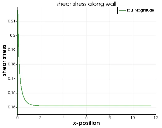
At the approximated length of 1.05 [m], wall shear stress gradient is considerably present. At a length of around 1.5[m], the gradients are quite negligible and `tau` becomes constant at around 1.8 [m]. This length of the pipe, where `tau` becomes constant, will be the entry length for this simulation which is considerably higher than our approximation using analytical equations.
3b. Fully developed velocity profile:
Velcity profiles along y-lines are plotted at various x positions in the domain. An analytical velocity profile is also computed in paraFoam using equ (1). `r` is computed using y-coordinate position in equ (1).
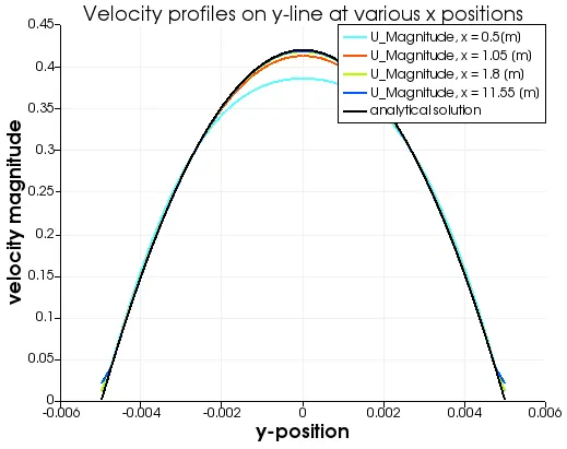
The velocity profiles at different x locations shows the velocity profile to develop at points, x = 0.5 [m], 1.05 [m] and becomes constant at around 1.8 [m]. This confirms our observation using wall shear stress. Fully developed velocity profile is formed at a length of 1.8 [m] and is maintained as constant until outlet of the pipe. This profile matches well with the analytical solution obtained using equ (1).
3c. Maximum velocity and pressure drop:
Maximum velocity of flow across the cross-section of pipe will occur at the axis of pipe due to least effect of viscosity. Velocity magnitude along the axis is plotted to see how the velocity varies and find the maximum velocity. Here the maximum velocity is seen to be 0.42 [m/s]
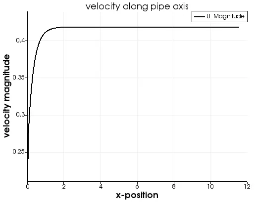
To find the average values of velocity and kinematic pressure at inlet and outlet, integrate variables filter is used on inlet and outlet patches separately.
 ----> inlet
 ----> outlet
The average kinematic pressure and velocity at inlet are found to be 0.8 [m^2/s^2] and 0.21 [m/s] respectively. Similarly, these values at outlet are found to be 0 [m^2/s^2] and 0.21 [m/s] respectively. So, average velocity across any cross-section along the pipe would be 0.21 [m/s]. Kinematic pressure drop across the pipe would be 0.8 [m^2/s^2]. Pressure drop in terms of gauge pressure can be obtained by multiplying this value by density of flowing medium, `rho`. Hence, pressure drop can be calculated as 800 [Pa].
Maximum velocity as deduced from analytical solution using equ (2), says it's twice the value of average velocity. The simulaiton also seems to confirm this calculation with `V_(avg)` = 0.21 [m/s] and `V_(max) = 2 * V_(Avg) = 0.42 [m//s]`
Analytical solution for pressure drop can be calculated using equ (3) as `Deltap = (32muLV_(avg))/D^2 = (32 * 10^-3 * 11.55 * 0.21)/0.01^2 = 776.16 [Pa]`. The pressure drop calculated using the simulation, 800 [Pa] is a good approximation of the analytical solution given that the entry length effects are not neglected in the simulation.
3d. Shear stress and wall shear stress.
Shear stress values as obtained above in paraFoam are plotted against y-lines in fully developed flow region.
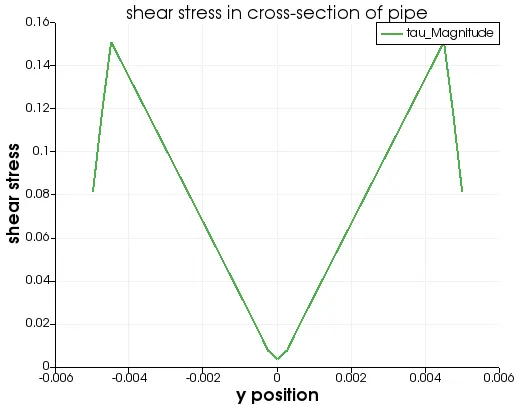
As expected, shear stress varies linearly from axis to walls of the pipe. Due to gradient algorithm used in paraFoam, shear stress values at the walls are shown incorrectly. Wall shear stress is approximated as shear stress values at 0.0045 [m] due to this limitation. Max shear stress values are felt at walls with minimum shear stress felt at the axis of the pipe flow where max flow velocity is experienced. Wall shear stress plot along the pipe is shown above which corresponds to the entry length of the pipe and beginning of fully developed flow profile.