Week 9 - FVM Literature Review
What is Finite Volume Method(FVM)?
Finite volume method (FVM) is based on the approximate solution of the integral form of the conservation equation. The problem domain is divided into a set of non overlapping control volumes called finite volumes. The conservation equation are applied to each finite volume. The integrals occuring in the conservation equations are evaluated using function values at computational nodes, which are usually taken as centroids of finite volumes. This process involves use of approximate integral formulae and interpolation methods to obtain the values of variables at surfaces of the CVs.
write down the major differences between FDM & FVM.
| FDM | FVM |
| This method cannot be used directly when the grids are not aligned along x,y,z direction. Therefore it is not suitabel for complex geometries. | This method can accomodate any type of grid and hence, it is naturally suitable for complex geometries. This method has immensly benefited from the unstructured grid generation methods developed for Finite element method. |
| The governing equation is valid only for grid points defined in the mesh | The governing equations is valid inside every point in the control volume. |
| It may or may not preserve the concept of conservation. | It always preserves the concept of conservation. |
The need for interpolation schemes and flux limiters in FVM:
The approximation of surface and volume integrals may require values of the variables at locations other than the computational nodes of the CV. Values at these locations are obtained using interpolation formulae.
Here control volume is defined as below:
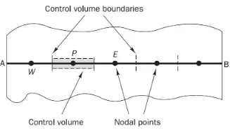
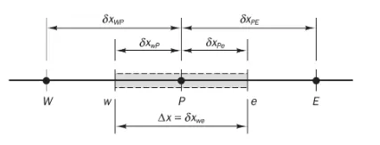
fig: Grid Generation
Here 1D linear heat conduction equation is defined in differential form which is converted into integral form as below:
`del/(delx)(alpha*(delT)/(delx))+S = 0`
where S is the source term in linear form.
The governing equation is valid for every point inside the control volume.
`int^P(del/(delx)(alpha*(delT)/(delx))+S )*delV= 0`
`int^Pdel/(delx)(alpha*(delT)/(delx))*dV+int^P S *dV= 0`
`int^Pdel/(delx)(alpha*(delT)/(delx))*A*dx+int^P S *dV= 0`
`[(alpha*A*(delT)/(delx))]_w^e + barS *dV= 0`
`alpha_e*A*((delT)/(delx))_e -alpha_w*A*((delT)/(delx))_w+ barS *dV= 0`
`alpha_e*A*[(T_E-T_P)/(Deltax)]-alpha_w*A**[(T_P-T_W)/(Deltax)]+ barS *dV= 0`
here value for `alpha_e and alpha_w` has to be determined using interpolation scheme as `alpha` is a function of temperature.
There are several methods to interpolate the value at different nodes other than the computational nodes.
Few of them are mentioned below:
- Upwind Interpolation Scheme(UDS):
The upwind Interpolation is used for approximating the value of a varibaale at the east face of the control volume given by
`fe = {fp if (v.n)_e>0`
`{ f_E if (v,n)_e<0`
This interpolation scheme is equivalent to using a backward or forward finite difference scheme, depending on the flow direction. It is first order accurate, and is numerically diffusive.
- Linear interpolation scheme:
We can also approximate the value of the variable at CV face center by linear interpolation of the values at two nearest computational nodes. Thus, at location 'e' on a cartesian grid, the vraible value id approximated by
`fe = f_E lamda_e +f_P(1-lamda_e)`
where
`lamda_e = (x_e-x_p)/(x_E-x_P)`
This method is equivalent to the use of central difference formua of the first order derivative, and hence, this scheme is also termed as central difference scheme(CDS). This scheme is second order accurate, and may produce oscillatory solutions.
- Quadratic upwind interpolation(QUICK):
This scheme can be derived using polynomial fitting. The QUICK interpolation on a uniform cartesian gird is given by
`phi_e = 6/8 phi_U + 3/8 phi_D - 1/8 phi_(UU)`
where D, U and UU denote the downstream, the first upstream and second upstream node respectively. QUICK scheme is third order accurate, but prone to oscillations.
Flux limiter:
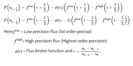
Flux limiters are used in the numerical schemes to solve highly coupled non-linear partial differential equations. If we tend to use low order numerical schemes for solving of the governing equations then we might get a highly oscillatory and unstable solution near the discoutinuity if present. whereas while using higher order numerical schemes to capture the phenomenon more accurately we tend to exploit the computational power unnecessarily. The main idea behind the use of the flux limiters is to limit the spatial derivative terms near the discontiuities to physical real values so as to maintain physcial consistency.
flux limiters are also referred to as slope limiters because they both have the same mathematical form, and both have the effect of limiting the solution gradient near shocks or discontinuites.
Mathematically,
Reference: