Week 5.1 - Mid term project - Solving the steady and unsteady 2D heat conduction problem
Steady state analysis & Transient State Analysis
Solve the 2D heat conduction equation by using the point iterative techniques that were taught in the class. The Boundary conditions for the problem are as follows;
Top Boundary = 600 K
Bottom Boundary = 900 K
Left Boundary = 400 K
Right Boundary = 800 K
To solve for dependent variables iterative techniques are used. Iterative solvers are:
- Jacobi iterative solver
- Gauss seidel interative solver
- Successive over relaxation iterative solver
2D heat conduction equation:
`(delT)/(delt) = alpha ((del^2T)/(delx^2)+(dela^2T)/(dely^2))`
The time derivative term is hyperbolic in nature which can be discretized using forward differencing scheme and the spatial derivatives are elliptical in nature which can be discretized using central differencing scheme.
Apply discretization we get,
`((del^2T)/(delx^2))_(i,j)^n = (T_((i+1),j)^n-2T_(i,j)^n+T_((i-1),j)^n)/(Deltax^2)`
`((del^2T)/(dely^2))_(i,j)^n = (T_(i,j+1)^n-2T_(i,j)^n+T_(i,j-1)^n)/(Deltay^2)`
Also
`((delT)/(delt))_(i,j)^n = (T_(i,j)^(n+1)-T_(i,j)^n)/(Deltat`
There the PDE becomes,
`(T_((i+1),j)^n-2T_(i,j)^n+T_((i-1),j)^n)/(Deltax^2) + (T_(i,j+1)^n-2T_(i,j)^n+T_(i,j-1)^n)/(Deltay^2)`=`(T_(i,j)^(n+1)-T_(i,j)^n)/(Deltat`
where n is current time step and n+1 is the next time step,
i, i+1 are neighbouring grid points in x direction, j,j+1 are the neighbouring grid points in y directions
Also, `Deltax` is grid spacing in x direction and `Delta y` is grid spacing in y direction
Iterative solvers:
1. Jacobi Iterative Solver
This method uses old values of temperature defined at previous time step n to find the new values at n+1 time step. Using the approximation obtained iteration is continued until the desired accuracy of the solution.
2. Gauss seidel Iterative solver
In this method, temperature at n+1 time step is calculated using both old value at n timestep and calculated value at n+1. BY this way the old approximated values are overwritten with new approximate values for iteration performed. Using updates value hepls for the solution to converge faster than the jacobi method
3. Succesive over relaxation
In this method, a relaxation factor is introduced which determines the rate of convergence of solution.
It is formulated as:
`T^(n+1) = t^n*(1-w)+w*T_(gs) or T_(jacobi)`
where w is the relaxation factor ranging from 0 to 2.
when w ranges from 0-1, it is called under relaxed state/
This condition is used when the temperature gradient is high and due to this time step doesnot overshoot and helps to converge faster.
similarly when w ranges from 1 -2, it is called over relaxed state.
This condition is used when the tempeature gradient is low and due to this larger time steps are used to obtain the steady state solition.
`T^n` is the value of temperature for previous iterations
`T_(gs) or T_(jacobi)` is the temperature value for n+1 th iteration obtained from iterative solvers.
There are two forms of heat conduction equation:
- Transient : `(delT)/(delt) = alpha ((del^2T)/(delx^2)+(dela^2T)/(dely^2))`
Discretization for transient heat equation:
`(T_(P)^(n+1)-T_(P)^n)/(Deltat)-alpha*((T_(L)^n-2T_(P)^n+T_(R)^n)/(Deltax^2) + (T_(P)^n-2T_(P)^n+T_(B)^n)/(Deltay^2))=0`
where
`T_p =T_(i,j)`
`T_L =T_(i-1,j)`
`T_R =T_(i+1,j)`
`T_T =T_(i,j+1)`
`T_B =T_(i,j-1)`
solving 2D transient heat conduction equation explicitly we get,
`T_p^(n+1) = (1-2*k1-2*k2)*T_p^n+k1*(T_L+T_R)^n+k2*(T_T+T_B)^n`
where, `k1 = alpha*(Deltat)/(Deltax^2)`
`k2 = alpha*(Deltat)/(Deltay^2)`
Stability criteria:
`k1+k2<=0.5`
Solving for 2D transient heat conduction equation implicitly we get
`T_p^(n+1) =( T_p^n+k1*(T_L+T_R)^(n+1)+k2*(T_T+T_B)^(n+1))/(1+2k1+2k2)`
here, n is for preceeding timestep and n+1 is the next timestep used for time integration.
Formula for jacobi iterative solver:
`T_p^(n+1) =( T_p^n+k1*(T_L+T_R)^(n)+k2*(T_T+T_B)^(n))/(1+2k1+2k2)`
Formula for gauss seidel iterative solver:
`T_p^(n+1) =( T_p^n+k1*(T_L^(n+1)+T_R^n)+k2*(T_T^n+T_B^(n+1)))/(1+2k1+2k2)`
Formula for successive over relaxation method:
`T_P^(n+1) = T_P^n*(1-w)+w*T_(gs) or T_(jacobi)`
Boundary conditions:
Boundary conditions are defined at the boundaries of independent variable of the function. In this problem mesh size of 10*10 is considered for which the boundary conditions are defined at corner rows and columns of the mesh.
| 500 | 600 | 600 | 600 | 600 | 600 | 600 | 600 | 600 | 700 |
|
400 |
300 | 300 | 300 | 300 | 300 | 300 | 300 | 300 | 800 |
| 400 | 300 | 300 | 300 | 300 | 300 | 300 | 300 | 300 | 800 |
| 400 | 300 | 300 | 300 | 300 | 300 | 300 | 300 | 300 | 800 |
| 400 | 300 | 300 | 300 | 300 | 300 | 300 | 300 | 300 | 800 |
| 400 | 300 | 300 | 300 | 300 | 300 | 300 | 300 | 300 | 800 |
| 400 | 300 | 300 | 300 | 300 | 300 | 300 | 300 | 300 | 800 |
| 400 | 300 | 300 | 300 | 300 | 300 | 300 | 300 | 300 | 800 |
| 400 | 300 | 300 | 300 | 300 | 300 | 300 | 300 | 300 | 800 |
| 650 | 900 | 900 | 900 | 900 | 900 | 900 | 900 | 900 | 850 |
- Steady : `(delta^2T)/(delta^2x)+(delta^2T)/(delta^2y)`
Discretization for steady state:
`((T_(L)^n-2T_(P)^n+T_(R)^n)/(Deltax^2) + (T_(T)^n-2T_(P)^n+T_(B)^n)/(Deltay^2))=0`
where
`T_p =T_(i,j)`
`T_L =T_(i-1,j)`
`T_R =T_(i+1,j)`
`T_T =T_(i,j+1)`
`T_B =T_(i,j-1)`
solving for T_p
`T_P^(n+1)=1/k((T_(L)^n+T_(R)^n)/(Deltax^2) + (T_(T)^n+T_(B)^n)/(Deltay^2))`
where, `k = 2*(Deltax^2+Deltay^2)/(Deltax^2*Deltay^2`
Solvinf the 2D steady heat conduction equation explicitly
Formula for Jacobi iterative solver:
`T_P^(n+1)=1/k((T_(L)^n+T_(R)^n)/(Deltax^2) + (T_(T)^n+T_(B)^n)/(Deltay^2))`
Formula for gauss seidel iterative solver:
`T_P^(n+1)=1/k*((T_(L)^(n+1)+T_(R)^(n+1))/(Deltax^2) + (T_(T)^(n+1)+T_(B)^(n+1))/(Deltay^2))`
Formula for successive over relaxation iterative solver:
`T_P^(n+1) = T_P^n*(1-w)+w*T_(gs) or T_(jacobi)`
Main program:
% program to study the behaviour of steady state and transient state
% analysis
clear all
close all
clc

%defining node
nx=10;
ny=10;

%length of the domain
L =1;
%calculating grid spacing
x = linspace(0,L,nx);
y = linspace(0,L,ny);
dx = x(2)-x(1);
dy = y(2)-y(1);

%initialize array and apply boundary conditions
t = 300*ones(nx,ny);
t(1:end,1)=400;  %left boundary
t(end,1:end) = 900;  %bottom boundary
t(1,1:end)= 600;   %top boundary
t(1:end,end) = 800;   %right boundary

%corner temperature
t(1,1) = (t(1,2)+t(2,1))/2;
t(end,1) = (t(end,2)+t((end-1)+1))/2;
t(1,end) = (t(2,end)+t(1,(end-1)))/2;
t(end,end) = (t((end-1),end)+t(end,(end-1)))/2;

%tolerance
tol = 1e-4;

%copy of initial temp matrix
told=t;
t_pre=t;

%coefficient from steady state equation
k = 2*(dx^2+dy^2)/(dx^2*dy^2);

%diffusivity coefficient in 2d heat conduction
alpha = 1.4;

%calculation of time step
dt = 0.5/((alpha/dx^2)+(alpha/dy^2));

% CFL terms
k1 = dt*alpha/dx^2;  %x term
k2 = dt*alpha/dy^2;  %y term

%relaxation factor for SOR for steady & transient heat conduction
w = 1.2;
w1 = 1.15;

%calling function to calculate the temperature of steady state using jacobi
%iterative solver
[error_j,iter1]=jacobi_iteration_steady(nx,ny,t,told,k,dx,dy,tol);

%calling function to calculate the temperature of steady state using gauss
%seidel iterative solver

[error_gs,iter2]=gausseidel_iteration_steady(nx,ny,t,told,k,dx,dy,tol);

%calling function to calculate the temperature of steady state using SOR
%iterative solver

[error_sor,iter3]=SOR_iteration_steady(nx,ny,t,told,k,dx,dy,tol,w);

%calling function to calculate the temperature of transient state using
%explicit method

[error_dt,iter_dt]=transient_heat_conduction(nx,ny,t,told,k1,k2);

%calling function to calculate the temperature of transient state using
%jacobi iterative solver

[error_j_2,iter_j_2]=transient_heat_conduction_j(nx,ny,t,t_pre,told,k1,k2,tol);

%calling function to calculate the temperature of transient state using
%gauss seidel iterative solver
[error_gs_2,iter_gs_2]=transient_heat_conduction_gs(nx,ny,t,t_pre,told,k1,k2,tol);

%calling function to calculate the temperature of transient state using
%SOR iterative solver

[error_sor_2,iter_sor]=SOR_iteration_unsteady(nx,ny,t,t_pre,told,k1,k2,tol,w1);
Jacobi Steady Iteration solver:
%function to calculate the temperature of steady state using jacobi
%iteration
function[error_j,iter1]=jacobi_iteration_steady(nx,ny,t,told,k,dx,dy,tol)

iter1 = 0;
error_j =9e9;

%convergence loop
while(error_j>tol)
    %iteration loop
        for i = 2:nx-1
            for j = 2:ny-1
                %formula to calculate temperature at each grid point
                t(i,j) = (1/k)*((told((i-1),j)+told((i+1),j))/dx^2)+(1/k)*((told(i,(j-1))+told(i,(j+1)))/dy^2);
            end
        end
        %error for each iter
        error1 = abs(told-t);
        error_j = max(error1,[],'all');

        %updating temperature values for next iteration
        told=t;
        iter1=iter1+1;
end
    %plotting the converged result
    figure(1)
    [C,h] = contourf(t);
    colormap(jet)
    colorbar
    set(gca,'YDIR','reverse')
    %labeling the plot here C represents temperature and h rotates the
    %temperature values as it moves
    clabel(C,h)
    axis ij;
    title('number of iteration for jacobi method for steady state heat conduction',iter1);
end
Gauss seidel Steady Iteration solver:
%function to calculate the temperature of steady state using gauss seidel
function[error_gs,iter2]=gausseidel_iteration_steady(nx,ny,t,told,k,dx,dy,tol)

iter2 = 0;
error_gs =9e9;

%convergence loop
while(error_gs>tol)
    %iteration loop
        for i = 2:nx-1
            for j = 2:ny-1
                %formula to calculate temperature at each grid point
                t(i,j) = (1/k)*((t((i-1),j)+t((i+1),j))/dx^2)+(1/k)*((t(i,(j-1))+t(i,(j+1)))/dy^2);
            end
        end
        %error for each iter
        error1 = abs(told-t);
        error_gs = max(error1,[],'all');

        %updating temperature values for next iteration
        told=t;
        iter2=iter2+1;
end
    %plotting the converged result
    figure(2)
    [C,h] = contourf(t);
    colormap(jet)
    colorbar
    set(gca,'YDIR','reverse')
    %labeling the plot here C represents temperature and h rotates the
    %temperature values as it moves
    clabel(C,h)
    pause(0.03)
    axis ij;
    title('number of iteration for gauss seidel method for steady state heat conduction',iter2);
end
SOR Steady Iteration solver:
%function to calculate the temperature of steady state using gauss seidel
function[error_sor,iter3]=SOR_iteration_steady(nx,ny,t,told,k,dx,dy,tol,w)

iter3 = 0;
error_sor =9e9;

%convergence loop
while(error_sor>tol)
    %iteration loop
        for i = 2:nx-1
            for j = 2:ny-1
                %formula to calculate temperature at each grid point
                t(i,j) = (1/k)*((t((i-1),j)+told((i+1),j))/dx^2)+(1/k)*((t(i,(j-1))+told(i,(j+1)))/dy^2);
                %SOR formula to calculate temperature
                t(i,j) = (1-w)*told(i,j)+w*t(i,j);

            end
        end
        %error for each iter
        error1 = abs(told-t);
        error_sor = max(error1,[],'all');

        %updating temperature values for next iteration
        told=t;
        iter3=iter3+1;
end
    %plotting the converged result
    figure(3)
    [C,h] = contourf(t);
    colormap(jet)
    colorbar
    set(gca,'YDIR','reverse')
    %labeling the plot here C represents temperature and h rotates the
    %temperature values as it moves
    clabel(C,h)
    axis ij;
    title('number of iteration for succesive over relaxation method for steady state heat conduction',iter3);
end
Transient explicit Iteration solver:
%function to calculate the temperature of unsteady/transient state using
%explicit method
function[error_dt,iter_dt]=transient_heat_conduction(nx,ny,t,told,k1,k2)

iter_dt = 0;
error_dt =9e9;

%time loop
for nt = 1:1400
    %iteration loop
        for i = 2:nx-1
            for j = 2:ny-1
                %formula to calculate temperature at each grid point
                H = told((i-1),j)-2*told(i,j)+told((i+1),j);    % temperature values in x-direction
                V = told(i,(j-1))-2*told(i,j)+told(i,(j+1));    % temperature values in y-direction
                % formula to calculate temperature
                t(i,j) = told(i,j)+k1*H+k2*V;

            end
        end
        %error for each iter
        error1 = abs(told-t);
        error_dt = max(error1,[],'all');

        %updating temperature values for next iteration
        told=t;
        iter_dt=iter_dt+1;
end
    %plotting the converged result
    figure(4)
    [C,h] = contourf(t);
    colormap(jet)
    colorbar
    set(gca,'YDIR','reverse')
    %labeling the plot here C represents temperature and h rotates the
    %temperature values as it moves
    clabel(C,h)
    axis ij;
    title('number of iteration using transient/unsteady state heat conduction explicitly',iter_dt);
end
Transient Gauss seidel Iteration solver:
%function to calculate the temperature of unsteady/transient state using
%gauss seidel
function[error_gs_2,iter_gs_2]=transient_heat_conduction_gs(nx,ny,t,t_pre,told,k1,k2,tol)

iter_gs_2 = 0;
error_gs_2 =9e9;
%error_f = 9e9;

%time loop
for nt = 1:1400
    %error_gs = 9e9;
    %convergence loop
    while(error_gs_2>tol)
        %space loop
        for i = 2:nx-1
            for j = 2:ny-1
                %formula to calculate temperature at each grid point
                term_1 = 1/(1+2*k1+2*k2);
                term_2 = k1*term_1;
                term_3 = k2*term_1;
                H = (t((i-1),j)+t((i+1),j));  %temperatue in x-direction
                V = (t(i,(j-1))+t(i,(j+1)));  %temperature in y-diection
                % formula to calculate temperature
                t(i,j) = term_1*t_pre(i,j)+term_2*H+term_3*V;
            end
        end
        %error for each iter
        %error1 = abs(told-t);
        %error_gs_2 = max(abs(told-t));
        error_gs_2 = max(max(abs(t_pre-t)));
        t_pre = t;
        %updating temperature values for next iteration
        %told=t;
        iter_gs_2=iter_gs_2+1;
    end

    %error_gs_2 = 9e9;
end
    %plotting the converged result
    figure(5)
    [C,h] = contourf(t);
    colormap(jet)
    colorbar
    set(gca,'YDIR','reverse')
    %labeling the plot here C represents temperature and h rotates the
    %temperature values as it moves
    clabel(C,h)
    axis ij;
    title('number of iteration for transient/unsteady state heat conduction using gauss seidel method ',iter_gs_2);
end
Transient Jacobi Iteration solver:
%function to calculate the temperature of unsteady/transient state using
%jacobi method
function[error_j_2,iter_j_2]=transient_heat_conduction_j(nx,ny,t,t_pre,told,k1,k2,tol)

iter_j_2 = 0;
error_j_2 =9e9;
%error_i= 9e9;

%time loop
for nt = 1:1400
    %convergence loop
    while(error_j_2>tol)
        %space loop
        for i = 2:nx-1
            for j = 2:ny-1
                %formula to calculate temperature at each grid point
                term_1 = 1/(1+2*k1+2*k2);
                term_2 = k1*term_1;
                term_3 = k2*term_1;
                H = (told((i-1),j)+told((i+1),j));  %temperatue in x-direction
                V = (told(i,(j-1))+told(i,(j+1)));  %temperature in y-diection
                % formula to calculate temperature
                t(i,j) = term_1*t_pre(i,j)+term_2*H+term_3*V;
            end
        end
        %error for each iter
        %error1 = abs(told-t);
        error_j_2 = max(max(abs(t_pre-t)));
        t_pre = t;
        %updating temperature values for next iteration
        told=t;
        iter_j_2=iter_j_2+1;
    end
    %error_i = max(max(abs(t_pre-t)));


end
    %plotting the converged result
    figure(6)
    [C,h] = contourf(t);
    colormap(jet)
    colorbar
    set(gca,'YDIR','reverse')
    %labeling the plot here C represents temperature and h rotates the
    %temperature values as it moves
    clabel(C,h)
    axis ij;
    title('number of iteration for transient/unsteady state heat conduction using jacobi method ',iter_j_2);
end
Transient SOR Iteration solver:
%function to calculate the temperature of steady state using SOR
function[error_sor_2,iter_sor]=SOR_iteration_unsteady(nx,ny,t,told,t_pre,k1,k2,tol,w1)

iter_sor = 0;
error_sor_2 =9e9;
%error_j = 9e9;

%time loop
for nt = 1:1400
    %convergence loop
    while(error_sor_2>tol)
    %iteration loop
        for i = 2:nx-1
            for j = 2:ny-1
                %formula to calculate temperature at each grid point
                term_1 = 1/(1+2*k1+2*k2);
                term_2 = k1*term_1;
                term_3 = k2*term_1;
                H = (t((i-1),j)+t((i+1),j));  %temperatue in x-direction
                V = (t(i,(j-1))+t(i,(j+1)));  %temperature in y-diection
                % formula to calculate temperature
                t(i,j) = w1*(t_pre(i,j)*term_1+term_2*H+term_3*V)+(1-w1)*t_pre(i,j);
               %t(i,j) = term_1*t_pre(i,j)+term_2*H+term_3*V;
                %SOR formula to calculate temperature
                %t(i,j) = (1-w1)*told(i,j)+w1*t(i,j);

            end
        end
        %error for each iter
        %error1 = abs(told-t);
        error_sor_2 = max(max(abs(t_pre-t)));
        t_pre = t;
        %updating temperature values for next iteration
        %told=t;
        iter_sor=iter_sor+1;
    end
    %error_j = max(max(abs(t_pre-t)));

    %error_sor_2 = 9e9;

end
    %plotting the converged result
    figure(7)
    [C,h] = contourf(t);
    colormap(jet)
    colorbar
    set(gca,'YDIR','reverse')
    %labeling the plot here C represents temperature and h rotates the
    %temperature values as it moves
    clabel(C,h)
    axis ij;
    title('number of iteration for succesive over relaxation method for unsteady state heat conduction',iter_sor);
end
Output graph:
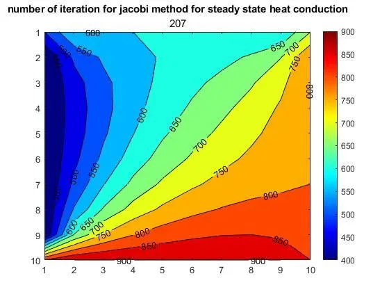
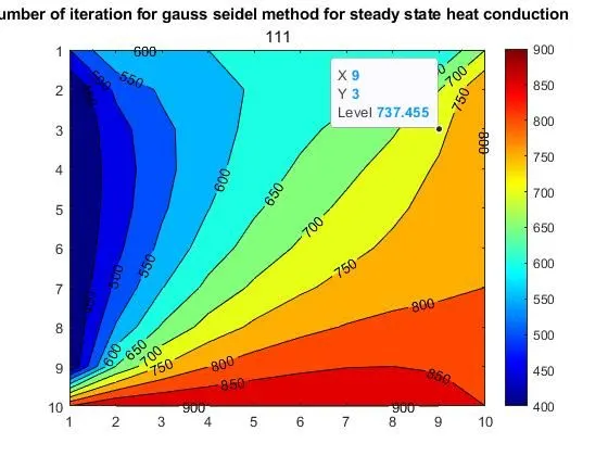
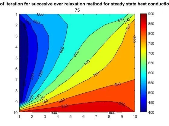
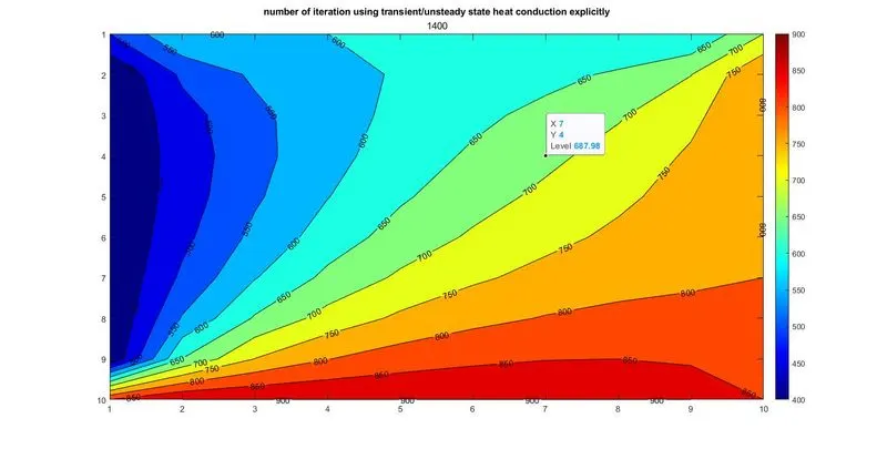
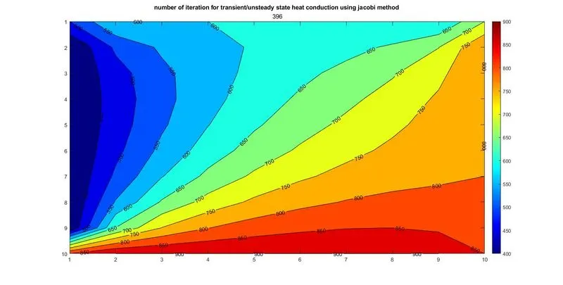
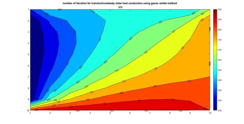
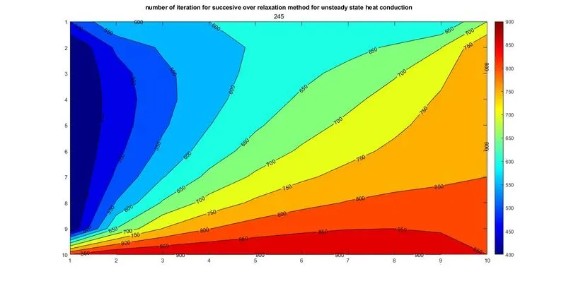
Table showing number of iterations required for each iterative solvers to converge:
Steady heat conduction equation:
| Iterative solver | No. of iterations |
|
Jacobi |
207 |
|
Gauss seidel |
111 |
|
SOR |
75 |
Transient heat conduction equation:
| Iterative solver | No. of iterations |
|
Jacobi |
396 |
|
Gauss seidel |
309 |
|
SOR |
245 |