Week 3.5 - Deriving 4th order approximation of a 2nd order derivative using Taylor Table method
Problem statement I : Derive the following 4th order approximations of the second-order derivative.
1. Central difference method
Consider a function f(x) whose 2nd order numerical derivative is given as
`f''(x) = (d^2f)/(d^2 t)`
We know,
The order of accuracy P = N - Q + 1 for symmetric/central schemes
where, N is Number of nodes in the stencil &
Q is order of derivative.
Then, N = P+Q-1
here, for 4th order approximations of the second order derivative.
P = 4
Q = 2
therefore, N = 5 ie, no of stencil node required for deriving central difference scheme is 5.
Now, defining a hypothetical second order derivative of f(x) at i using central difference scheme
`(del^2f)/(del^2x) = a*f(i-2) + b*f(i-1)+c*f(i)+d*f(i+1)+e*f(i+2)`
where, a,b,c,d and e are approximation coefficients.
let `Delta x`be discretization size or grid spacing then the taylor expansion of a*f(i-2) is
`a*f(i-2)` = `a [ f(i) - 2Deltax*f'(i)+(2Delta)^2/(2!)*f''(i)-(2Delta)^3/(3!)*f'''(i)+(2Delta)^4/(4!)*f^(iv)(i)-(2Delta)^5/(5!)*f^(v)(i)+(2Delta)^6/(6!)*f^(vi)(i)+....]`
similarly for 2nd term,
`b*f(i-1)`= `a [ f(i) - Deltax*f'(i)+(Delta)^2/(2!)*f''(i)-(Delta)^3/(3!)*f'''(i)+(Delta)^4/(4!)*f^(iv)(i)-(Delta)^5/(5!)*f^(v)(i)+(Delta)^6/(6!)*f^(vi)(i)+....]`
similarly,
`c*f(i) = c*f(i)`
similarly,
`d * f(i+1)`= `a [ f(i) + Deltax*f'(i)+(Delta)^2/(2!)*f''(i)+(Delta)^3/(3!)*f'''(i)+(Delta)^4/(4!)*f^(iv)(i)+(Delta)^5/(5!)*f^(v)(i)+(Delta)^6/(6!)*f^(vi)(i)+....]`
similarly,
`e*f(i+2)` = `a [ f(i) +2Deltax*f'(i)+(2Delta)^2/(2!)*f''(i)+(2Delta)^3/(3!)*f'''(i)+(2Delta)^4/(4!)*f^(iv)(i)+(2Delta)^5/(5!)*f^(v)(i)+(2Delta)^6/(6!)*f^(vi)(i)+....]`
Above terms can be represented in tabular form known as taylor's table as given below
| `f(i)` | `Deltax*f'(i)` | `Deltax^2*f''(i)` | `Deltax^3*f'''(i)` | `Deltax^4*f^(iv)(i)` | `Deltax^5*f^(v)(i)` | `Deltax^6*f^(vi)(i)` | |
| `a*f(i-2)` | a | -2a | `(4a)/2` | `-(8a)/2` | `2a/3` | `-(4a)/15` | `4a/15' |
| `b*f(i-1)` | b | -b | `b/2` | `-b/6` | `b/24` | `-b/120` | `b/720` |
| `c*f(i)` | c | 0 | 0 | 0 | 0 | 0 | 0 |
| `d * f(i+1)` | d | d | `d/2` | `d/6` | `d/24` | `d/120` | `d/720` |
| `e*f(i+2)` | e | 2e | `(4e)/2` | `(8e)/6` | `(2e)/3` | `(4e)/15` | `(4e)/45` |
| `(del^2f)/(del^2x)`= sum of all above terms | 0 | 0 | 1 | 0 | 0 | ? |
? |
Here only the second order derivative terms sum is eqaul to 1 and rest all are zero. The last two columns are neglected as we require only five equations to find out the five unknown.
Now, summing above
`a+b+c+d+e=0`
`-2a-b+d+2e=0`
`(4a)/2+b/2+d/2+(4e)/2=1`
`(-8a)/6-b/6+d/6+(8e)/6=0`
`(2a)/3+b/24+d/24+(2e)/3=0`
converting above system of equation into matrix form:
`[[1,1,1,1,1],[-2,-1,0,1,2],[2,1/2,0,1/2,2],[-8/6,-1/6,0,1/6,8/6],[2/3,1/24,0,1/24,2/3]] [[a],[b],[c],[d],[e]] = [[0],[0],[1],[0],[0]]`
solving the matrix by inversion leads to
a = `-1/12`
b = `4/3`
c = `-5/2`
d = `4/3`
e = `-1/12`
here we can see, a = e & b=d
substituting the value in the hypothesis equation along with taylor series expansion of each term,
`(del^2f)/(del^2x) = a*f(i-2) + b*f(i-1)+c*f(i)+d*f(i+1)+e*f(i+2) = 0+0+1*f^(ii) Deltax^2+0+0+((8a)/45+b/360)*f^(vi) Deltax^6`
dividing both sides by `Deltax^2` and rewriting as
`(del^2f)/(del^2x) = (a*f(i-2) + b*f(i-1)+c*f(i)+d*f(i+1)+e*f(i+2) )/(Deltax^2)= f^(ii) +((8a)/45+b/360)*f^(iv) Deltax^4`
Hence, the above equation represents the fourth order central difference approximation for second derivative and here the terms with 4th order is neglected to get the result therefore the truncation error is of fourth order.
therefore,
`(del^2f)/(del^2x) = (a*f(i-2) + b*f(i-1)+c*f(i)+d*f(i+1)+e*f(i+2) )/(Deltax^2) ............`(1)
2. Skewed right-sided difference
We know,
The order of accuracy P = N - Q for skewed schemes
where, N is Number of nodes in the stencil &
Q is order of derivative.
Then, N = P+Q
here, for 4th order approximations of the second order derivative.
P = 4
Q = 2
therefore, N = 6 ie, no of stencil node required for deriving central difference scheme is 6.
Now, defining a hypothetical second order derivative of f(x) at i using skewed scheme
`(del^2f)/(del^2x) = g*f(i)+h*f(i+1)+j*f(i+2)+k*f(i+3)+l*f(i+4)+m*f(i+5)`
where, g,h,i,j,k & lare approximation coefficients.
let `Delta x`be discretization size or grid spacing then the taylor expansion of h*f(i+1) is
`h * f(i+1)`= `h [ f(i) + Deltax*f'(i)+(Delta)^2/(2!)*f''(i)+(Delta)^3/(3!)*f'''(i)+(Delta)^4/(4!)*f^(iv)(i)+(Delta)^5/(5!)*f^(v)(i)+(Delta)^6/(6!)*f^(vi)(i)+....]`
similarly,
`j*f(i+2)` = `j [ f(i) +2Deltax*f'(i)+(2Delta)^2/(2!)*f''(i)+(2Delta)^3/(3!)*f'''(i)+(2Delta)^4/(4!)*f^(iv)(i)+(2Delta)^5/(5!)*f^(v)(i)+(2Delta)^6/(6!)*f^(vi)(i)+....]`
similarly,
`k*f(i+3) =k [ f(i) +3Deltax*f'(i)+(3Delta)^2/(2!)*f''(i)+(3Delta)^3/(3!)*f'''(i)+(3Delta)^4/(4!)*f^(iv)(i)+(3Delta)^5/(5!)*f^(v)(i)+(3Delta)^6/(6!)*f^(vi)(i)+....]`
similarly,
`l*f(i+3) =l[ f(i) +4Deltax*f'(i)+(4Delta)^2/(2!)*f''(i)+(4Delta)^3/(3!)*f'''(i)+(4Delta)^4/(4!)*f^(iv)(i)+(4Delta)^5/(5!)*f^(v)(i)+(4Delta)^6/(6!)*f^(vi)(i)+....]`
similarly,
`m*f(i+3) =m [ f(i) +5Deltax*f'(i)+(5Delta)^2/(2!)*f''(i)+(5Delta)^3/(3!)*f'''(i)+(5Delta)^4/(4!)*f^(iv)(i)+(5Delta)^5/(5!)*f^(v)(i)+(5Delta)^6/(6!)*f^(vi)(i)+....]`
Above terms can be represented in tabular form known as taylor's table as given below
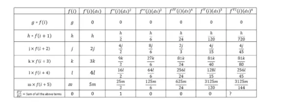
Here only the second order derivative terms sum is eqaul to 1 and rest all are zero. The last column is neglected as we require only six equations to find out the six unknown.
Now, summing above
`g+h+j+k+l+m=0`
`h+2j+3k+4l+5m=0`
`h/2+4j/2+9k/2+16l/2+25m/2=1`
`h/6+8j/6+27k/6+64l/6+125m/6=0`
`h/24+2j/3+81k/24+256l/24+625m/24=0`
`h/120+4j/15+81k/40+128l/15+3125m/120=0`
converting the above into matrix form:
`[[1,1,1,1,1,1],[0,1,2,3,4,5],[0,1/2,4/2,9/2,16/2,25/2],[0,1/6,8/6,27/6,64/6,125/6],[0,1/24,2/3,81/24,256/24,625/24],[0,1/120,4/15,81/40,128/15,3125/120]][[g],[h],[j],[k],[l],[m]] = [[0],[0],[1],[0],[0],[0]]`
solving by matrix inversion
g = 15/4
h = -77/6
j = 107/6
k = -13
l = 61/12
m = -5/6
substituting these values in the taylor table leads all terms to zero except column 4 and 8.
rewriting the hypothesis equation in terms of taylor series expansion of individual terms:
`(del^2f)/(del^2x) = g*f(i)+h*f(i+1)+j*f(i+2)+k*f(i+3)+l*f(i+4)+m*f(i+5) = 0+0+1*f^(ii)Delta^2 +0+0+0+(h/720+4j/45+81k/80+256l/45+3125m/44)*f^(vi)(i+6)Delta^6`
`(del^2f)/(del^2x) = (g*f(i)+h*f(i+1)+j*f(i+2)+k*f(i+3)+l*f(i+4)+m*f(i+5))/(Deltax^2)= F^(ii)(i)+O*Deltax^4`
Hence, the above equation represents the fourth order central difference approximation for second derivative and here the terms with 4th order is neglected to get the result therefore the truncation error is of fourth order.
therefore,
`(del^2f)/(del^2x) = (g*f(i)+h*f(i+1)+j*f(i+2)+k*f(i+3)+l*f(i+4)+m*f(i+5))/(Deltax^2)`
3. Skewed left-sided difference
We know,
The order of accuracy P = N - Q for skewed schemes
where, N is Number of nodes in the stencil &
Q is order of derivative.
Then, N = P+Q
here, for 4th order approximations of the second order derivative.
P = 4
Q = 2
therefore, N = 6 ie, no of stencil node required for deriving central difference scheme is 6.
Now, defining a hypothetical second order derivative of f(x) at i using skewed scheme
`(del^2f)/(del^2x) = n*f(i-5)+p*f(i-4)+q*f(i-3)+r*f(i-2)+s*f(i-1)+t*f(i)`
where, n,p,q,r,s & t are approximation coefficients.
Expanding all terms of the hypothetical equation using taylor series expansion and representing it in form of table using taylor table method.
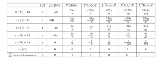
Here only the second order derivative terms sum is eqaul to 1 and rest all are zero. The last column is neglected as we require only six equations to find out the six unknown.
Now summing above,
`n+p+q+r+s+t=0`
`-5n-4p-3q-2r-s=0`
`25n/2+a6p/2+9q/2+4r/2+s/2=1`
`-125n/6-64p/6-27q/6-8r/6-s/6=0`
`625n/24+256p/24+81q/24+2r/3+s/24=0`
`-3125n/120-128p/15-81q/40-4r/15-s/120=0`
converting into matrix form:
`[[1,1,1,1,1,1],[-5,-4,-3,-2,-1,-0],[25/2,16/2,9/2,4/2,1/2,0],[-125/6,-64/6,-27/6,-8/6,-1/6,0],[625/24,256/24,81/24,2/3,1/24,0],[-3125/120,-128/15,-81/40,-4/15,-1/120,0]][[n],[p],[q],[r],[s],[t]] = [[0],[0],[1],[0],[0],[0]]`
solving the matrix by inversion method, we get
n = -5/6
p = 61/12
q = -13
r = 107/6
s = -77/6
t = 15/4
substituting these values in the taylor table leads all terms to zero except column 4 and 8.
rewriting the hypothesis equation in terms of taylor series expansion of individual terms:
`(del^2f)/(del^2x) = n*f(i-5)+p*f(i-4)+q*f(i-3)+r*f(i-2)+s*f(i-1)+t*f(i)=0+0+1*f''(i)Deltax^2+0+0+0+(3125n/144+256p/45+81q/80+4r/45+s/720)*f^(vi)(i)Deltax^6+....`
dividing both sides by `Deltax^2` and rewriting as
`(del^2f)/(del^2x) = n*f(i-5)+p*f(i-4)+q*f(i-3)+r*f(i-2)+s*f(i-1)+t*f(i)=f''(i)+ODeltax^4`
Hence, the above equation represents the fourth order central difference approximation for second derivative and here the terms with 4th order is neglected to get the result therefore the truncation error is of fourth order.
`(del^2f)/(del^2x) = (n*f(i-5)+p*f(i-4)+q*f(i-3)+r*f(i-2)+s*f(i-1)+t*f(i))/(Deltax^2)....`
Problem II:
- To write a program in Matlab to evaluate the second-order derivative of the analytical function exp(x)*cos(x) and compare it with the 3 numerical approximations derived from fourth-order accuracy.
- To plot the graph that compares the absolute error between the above-mentioned schemes
Matlab code:
Function using central differencing:
function out = fourth_order_central_differencing(x,dx)

%analytical function = exp(x)*cos(x)
%analytical derivative is f''(x)=-2*exp(x)*sin(x);
analytical_derivative = -2*exp(x)*sin(x);


%approximation coefficients
a = -1/12;

b = 4/3;

c = -5/2;

d = 4/3;

e = -1/12;

%numerical derivative using central differencing scheme

central_differencing = ((a*((exp(x-(2*dx)))*cos(x-(2*dx))))+(b*((exp(x-dx)))*(cos(x-dx)))+(c*(exp(x)*cos(x)))+(d*(exp(x+dx))*(cos(x+dx)))+(e*(exp(x+(2*dx)))*(cos(x+(2*dx)))))/((dx)^2);

%absolute error
out = abs(central_differencing-analytical_derivative);
end
function using right sided skewed :
function out = fourth_order_right_skewed(x,dx)

%analytical function = exp(x)*cos(x)
%analytical derivative is f''(x)=-2*exp(x)*sin(x);
analytical_derivative = -2*exp(x)*sin(x);


%approximation coefficients
g = 15/4;
h = -77/6;
j = 107/6;
k = -13;
l = 61/12;
m = -5/6;
%numerical derivative using skewed right sided differencing

right_sided_skewed =((g*exp(x)*cos(x))+(h*exp(x+dx)*cos(x+dx))+(j*exp(x+(2*dx))*cos(x+(2*dx)))+(k*exp(x+(3*dx))*cos((x+(3*dx))))+(l*exp(x+(4*dx))*cos(x+(4*dx)))+(m*exp(x+(5*dx))*cos(x+(5*dx))))/((dx)^2);

%absolute error
out = abs(right_sided_skewed-analytical_derivative);

end
function using left sided skewed :
function out = fourth_order_left_skewed(x,dx)

%analytical function = exp(x)*cos(x)
%analytical derivative is f''(x)=-2*exp(x)*sin(x);
analytical_derivative = -2*exp(x)*sin(x);

%approximation coefficients
n = -5/6;
p = 61/12;
q = -13;
r = 107/6;
s = -77/6;
t = 15/4;

%numerical derivative using fourth order left skewed differencing

left_sided_skewed = ((n*exp(x-(5*dx))*cos(x-(5*dx)))+(p*exp(x-(4*dx))*cos(x-(4*dx)))+(q*exp(x-(3*dx))*cos(x-(3*dx)))+(r*exp(x-(2*dx))*cos(x-(2*dx)))+(s*exp(x-dx)*cos(x-dx))+(t*exp(x)*cos(x)))/((dx)^2);

%absolute error
out = abs(left_sided_skewed -analytical_derivative);
end
main function to compare error between above scheme:
%main code
clear all
close all
clc

% value of x
x = pi/3;

%range of dx
dx = linspace(pi/400,pi/40,20);

for i = 1:length(dx)

    central_differencing(i) =fourth_order_central_differencing(x,dx(i));
    right_sided_skew(i) = fourth_order_right_skewed(x,dx(i));
    left_sided_skew(i) = fourth_order_left_skewed(x,dx(i));

end

%plot of dx and error

figure(1)
loglog(dx,central_differencing,'linewidth',2,'marker','o')
hold on
loglog(dx,right_sided_skew,'linewidth',2,'marker','x')
hold on
loglog(dx,left_sided_skew,'linewidth',2,'marker','square')
xlabel('range of dx')
ylabel('truncation error')
title('range of dx vs error')
legend('central differencing','skewed right sided differencing','skewed right sided differencing','location','northwest')
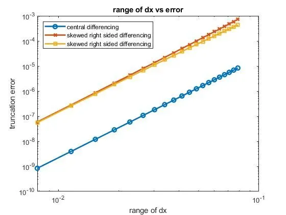
Output:
Conclusion:
As seen from the plot we can conclude that the central differencing scheme has very less error in comparison with the skewed scheme. Therefore, central differencing scheme is better than other schemes because it uses informatin from the both sides of the stencil to give better results.
Why a skewed scheme is useful?
Sometimes a system under consideration may not contain sufficient information on both sides of the point of interest. In such cases we are not able to use central differencing scheme therefore skewed scheme is useful in such cases.
What can a skewed scheme do that a CD scheme cannot?
CD scheme cannot be used at the boundary nodes because at boundary nodes both the right and left nodes are not available at the same time. In such cases the skewed scheme is used.