Week 7 - Simulation of a 1D Super-sonic nozzle flow simulation using Macormack Method

Problem statement:

1. Simulate the isentropic flow through a quasi 1D subsonic-supersonic nozzle.
2. Derive both the conservation and non-conservation forms of the governing equations and sovle them using the MacCormack's technique.
3. Determine the steady-state temperature distribution for the flow-field variables and investigate the difference between the two forms of governing equations by comparing their solutions.
4. Perform a grid independence test on the solution

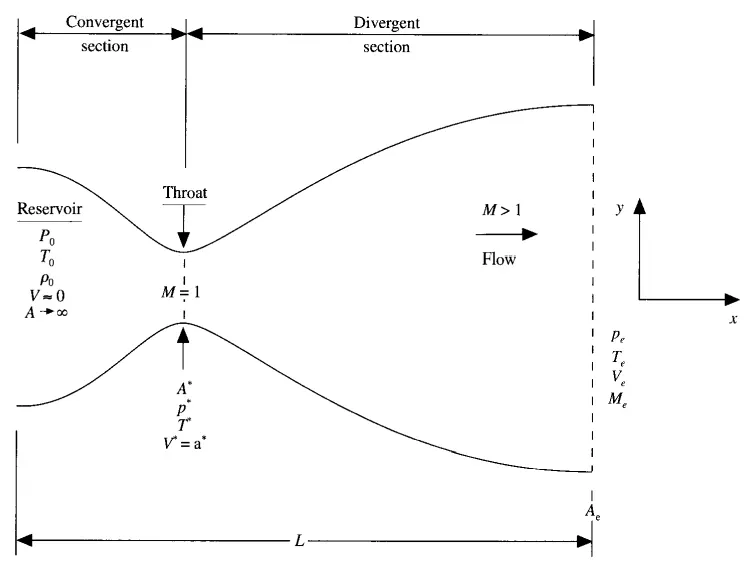
Schematic for quasi 1D subsonic-supersonic isentropic nozzle flow:

The Governing flow equations:

Conservative form:

• Continuity equation:

`del/dt(rhoA)+del/delx(rhoAv) = 0`

• Momentum equation:

`del/(delt) (rhoAv)+del/(delx)(rhoAv^2)=-A(delp)/(delx)`

• Energy equation:

`del/(delt)(rho/2v^2A)+del/(delx)(rhov^3/2A) = -Av(delp)/(delx)`

where,

`rho` = density

v = velocity of flow

A = cross sectional area of nozzle

p = pressure

all the variables above are in non dimensional form:

`rho' = rho/rho_o`

similarly other variables are taken in reference to their reserviour values.

Inorder to solve the conservation form of governing equation using computational method, above equation is defined in terms solution vector, flux vector and source term. Only solving continuity equation for simplicity.

• Solution vectors:

`u1 = rho*A`

`u2 = rho*A*v`

`u3 = rho(t/(gamma-1)+gamma/2 * v^2)A`

• Flux terms:

`f1 = u2`

`f2 = (u2^2)/(u1)+(gamma-1)/gamma * (u3-gamma/2*(u2^2)/(u1))`

`f3 = gamma*((u2*u3)/(u1))-gamma/2*(gamma-1)*(u2^3)/(u1^2)`

• Source term:

`j2 = 1/gamma*rho*t*(delA)/(delx)`

Therefore,

• Continuity equation in terms of above terms:

`(delu1)/dt = -(delf1)/(delx)`

• Momentum equation:

`(delu2)/(delx) = -(delf2)/(delx)+j2`

• Energy equation:

`(delu3)/(delt) = -(delf2)/(delx)`

Now these pure form of governing equation is used to find the primitive variables in the nozzle domain using maccormack's technique. It is a predictor-corrector method of 2nd order accuracy.

1. Predictor step

Here, the space derivative term i.e flux term is discritized using forward differencing scheme

`((delf1)/dx) _j^t= (f1^t(j+1)-f1^t(j))/(Deltax)`

Here the terms are defined in the time step t.

Continuity equation:

`((du1)/dt)_p^t = -((df1)/dx)_j^t`

b. Solution update:

`(u1)_j^(t+Deltat) = (u1)_j^t +((du1)/dt)_p^t*Deltat`

c. Corrector step:

Here, the space derivative term i.e flux term is discritized using backward differencing scheme

`((df1)/dx)_(j)^(t+Deltat) = (f1^(t+Deltat)(j)-f1^(t+Deltat)(j-1))/(Deltax)`

Similarly

`((du1)/dt)_j^(t+Deltat) = -((df1)/dx)_j^(t+Deltat)`

Finding average value,

`( (du1)/dt)_(avg) = 0.5*[((du1)/dt)_p^t+((du1)/dt)_j^(t+Deltat)]`

d. Final solution update:

`u1_(j) ^(t+Deltat)= u1(old)_(f)^t+((du1)/dt)_(avg)*Deltat`

The primitive values are calculated from above final solution as

`rho = (u1)/A`

`v = (u2)/(u1)`

`T = (gamma-1)((u3)/(u2)-gamma/2v^2)`

Non-conservation form:

Inorder to solve the governing equation using computational method, non dimensional form of equation is used.

Non-dimensional form:

• Continuity equation:

`(drho)/dt = -rho(delv)/(delx)-rhov(del(lnA))/dx -v(drho)/dx`

• Momentum equation:

`(dv)/dt = -v(dv)/dx - (1/gamma)*((dT)/dx+T/rho*(drho)/dx)`

• Energy equation:

`(delT)/(delt) = -v*(delT)/(delx)-(gamma-1)*T*((dv)/dx+v*(del(loga))/dx)`

Now these equation is solved using maccormack's technique similar to above process for the conservative part.

1. Predictor step:

Here the space derivative term is discretized using forward differencing scheme

`(delv)/(delx) = (v(j+1)-v(j))/(Deltax)`

`(delrho)/(delx) = (rho(j+1)-rho(j))/(Deltax)`

`(delT)/(delx) = (T(j+1)-T(j))/(Deltax)`

`(delloga)/(delx )= (log(a(j+1))-log(a(j)))/(Deltax)`

Replacing above terms in each governing equation. Here solving only for density for simplicity.

For continuity equation:

`((drho)/dt)_p^t = -rho(delv)/(delx)-rhov(del(lnA))/dx -v(drho)/dx`

ii. Solution update:

`rho_(j) = rho_(j) + (((drho)/dt)_p^t*Deltat)`

iii. Corrector step:

Here the space derivative term is discretized using backward differencing scheme.

`(delv)/(delx) = (v(j)-v(j-1))/(Deltax)`

`(delrho)/(delx) = (rho(j)-rho(j-1))/(Deltax)`

`(delT)/(delx) = (T(j)-T(j-1))/(Deltax)`

`(delloga)/(delx )= (log(a(j))-log(a(j-1)))/(Deltax)`

These discretized term are again replaced in the governing equation

`((drho)/dt)_c^(t+Deltat) = -rho(delv)/(delx)-rhov(del(lnA))/dx -v(drho)/dx`

Finding the average value:

`((delrho)/(delt))_(avg) = 0.5*(((drho)/dt)_p^t +((drho)/dt)_c^(t+Deltat))`

iv. Final solution update:

`rho_(j) = rho__old _(j) + (((drho)/dt)_(avg,j)^t*Deltat)`

Calculation of time step:

The formula used to calculate time step is

`Delta t = C*(Deltax)/(a+V)`

where,

C is courant number

x is grid size

a is speed of sound

V is flow speed

The time step can be calculated using two approach for the time marching solution.

1. Utilizing local values of `Delta t` at each grid point i. In this fashion, the flow field variables at each grid point will be advanced in time according to their own, local time step. Using local time step will frequently lead to faster convergence to the steady state. But local time stepping method may not lead to correct steady state in every scenarios.
2. The other approach is to calculate `(Deltat)_i^t` at all grid points from i =1 to i = n and to choose the minimum value for use in solution update step.

`Delta t =`minimum (`(Delta t)_1^t, (Delta t)_2^t,(Delta t)_3^t, .....(Delta t)_i^t,.....(Delta t)_n^t,`

Using second approach is more reasonable.

Main program to calculate result for both forms of governing equations:

clear all
close all
clc

%inputs
n = 31;
x = linspace(0,3,n);
dx = x(2) - x(1);
gamma =1.4; 

tic
%calling non conservative form of governing eqauation to plot the primitive
%values
[ rho, v, t,k,m_t,t_th,pr_th,mach_th,rho_th,v_th] = non_conservative(x,n,gamma,dx);
time_nc = toc;
tic 
%calling conservative form of governing eqauation to plot the primitive
%values
[rho_c, v_c, t_c,m_c,t_th_c,pr_th_c,mach_th_c,rho_th_c,v_th_c] = conservative_final(x,n,gamma,dx);
time_c = toc;
%defining the exact value of variables
rho_exact = 0.634*ones(1,1400);
t_exact = 0.833*ones(1,1400);
p_exact = 0.528*ones(1,1400);
Mach_exact = 1*ones(1,1400);

%plot for the non conservation form plotting for variables at throat

figure(1)
subplot(4,1,1)
plot(t_th,'linewidth',2)
hold on
xlabel('time')
ylabel('t/t_0')
title(["plot of variables at throat for non conservative form";"plot of temperature at thorat"])
legend('time wise variation');

subplot(4,1,2)
plot(rho_th,'linewidth',2)
hold on 
xlabel('time')
ylabel('rho/rho_0')
title('plot of density at throat')
legend('time wise variation');

subplot(4,1,3)
plot(pr_th,'linewidth',2)
hold on 
xlabel('time')
ylabel('pr/pr_0')
title('plot of pressure values at throat')
legend('time wise variation');

subplot(4,1,4)
plot(mach_th,'linewidth',2)
hold on 
xlabel('time')
ylabel('M/M_0')
title('plot of mach number at throat')
legend('time wise variation');

%plotting of steady state distribution primitive variables inside domain
figure(2)
%plot for density
subplot(3,1,1)
plot(x,rho,'linewidth',1)
xlabel('nozzle domain')
ylabel('density')
title(["Plot of steady state distribution of primitive variables inside nozzle domain for non conservation form";"density variation inside nozzle domain"])
axis([0.5 3 0 max(rho)])

%plot for temperature
subplot(3,1,2)
plot(x,t,'linewidth',1)
xlabel('nozzle domain')
ylabel('temperature')
title('temperature variation inside nozzle domain')
axis([0.5 3 0 max(t)])

%plot for velocity
subplot(3,1,3)
plot(x,v,'linewidth',1)
xlabel('nozzle domain')
ylabel('velocity')
title('density variation inside nozzle domain')
axis([0.5 3 0 max(v)])


%plot for the conservation form plotting for variables at throat

figure(4)
subplot(4,1,1)
plot(t_th_c,'linewidth',2)
hold on
%plot(t_exact,'linewidth',2,'g')
xlabel('time')
ylabel('t/t_0')
title(["plot of variables at throat for conservative form";"plot of temperature at thorat"])
legend('time wise variation');

subplot(4,1,2)
plot(rho_th_c,'linewidth',2)
hold on 
%plot(rho_exact,'linewidth',2,'g')
xlabel('time')
ylabel('rho/rho_0')
title('plot of density at throat')
legend('time wise variation');

subplot(4,1,3)
plot(pr_th_c,'linewidth',2)
hold on 
%plot(pr_exact,'linewidth',2,'g')
xlabel('time')
ylabel('pr/pr_0')
title('plot of pressure values at throat')
legend('time wise variation');

subplot(4,1,4)
plot(mach_th_c,'linewidth',2)
hold on 
%plot(mach_exact,'linewidth',2,'g')
xlabel('time')
ylabel('M/M_0')
title('plot of mach number at throat')
legend('time wise variation');

%plotting of steady state distribution primitive variables inside domain
figure(5)
%plot for density
subplot(3,1,1)
plot(x,rho_c,'linewidth',1)
xlabel('nozzle domain')
ylabel('density')
title(["Plot of steady state distribution of primitive variables inside nozzle domain for conservation form";"density variation inside nozzle domain"])
axis([0.5 3 0 max(rho_c)])

%plot for temperature
subplot(3,1,2)
plot(x,t_c,'linewidth',1)
xlabel('nozzle domain')
ylabel('temperature')
title('temperature variation inside nozzle domain')
axis([0.5 3 0 max(t_c)])

%plot for velocity
subplot(3,1,3)
plot(x,v_c,'linewidth',1)
xlabel('nozzle domain')
ylabel('velocity')
title('density variation inside nozzle domain')
axis([0.5 3 0 max(v_c)])

figure(8)
plot(x,m_c)
hold on
plot(x,m_t)
title_text = sprintf('Normalized Mass Flow rate distribution inside nozzle domain for %d grid points',n);
title(title_text)
legend('Conservative','Non-conservative')
xlabel('nozzle domain')
ylabel('mass flow rate m')

Function to calculate non conservative form of governing equation:

function [rho, v, t,k,m_t,t_th,pr_th,mach_th,rho_th,v_th] = 
non_conservative(x,n,gamma,dx)

%calculate intial profiles
rho = 1 - 0.3146*x;
t = 1 - 0.2314*x;
v = (0.1+1.09*x).*(t.^(0.5));
%area
a = 1+(2.2)*((x-1.5).^2);

thr = find(a==1);
%no of time steps
nt = 1400;
dt1 = 0.5*(dx./(sqrt(t)+v));
dt = min(dt1);

%outer time loop
for k = 1:nt
    rho_old = rho;
    v_old = v;
    t_old = t;
    
    %predictor method
    
    for j = 2 : n-1
        %drho_dt_p = -rho(j)*((v(j+1)-v(j)))/dx-rho(j)*v(j)*((log(A(j+1))-log(A(j))))/dx-v(j)*((rho(j+1)-rho(j)))/dx;
        dvdx = (v(j+1)-v(j))/dx;
        drhodx = (rho(j+1)-rho(j))/dx;
        dtdx = (t(j+1)-t(j))/dx;
        dlogadx = (log(a(j+1))-log(a(j)))/dx;
              
        %continuity equation
        drho_dt_p(j) = -rho(j)*(dvdx) - rho(j)*v(j)*(dlogadx)-(v(j)*drhodx);
        
        %momentum eqaution
        dvdt_p(j) = -(v(j)*dvdx) - (1/gamma)*(dtdx+(t(j)/rho(j))*drhodx);
        
        %energy equation
        dtdt_p(j) = -v(j)*(dtdx)-(gamma-1)*t(j)*(dvdx+v(j)*dlogadx);
        
        %solution update
        
        rho(j) = rho(j) + (drho_dt_p(j)*dt);
        v(j) = v(j) + (dvdt_p(j)*dt);
        t(j) = t(j) + (dtdt_p(j)*dt);
        
    end
    %corrector step
    for j = 2 : n-1
        %drho_dt_p = -rho(j)*((v(j+1)-v(j)))/dx-rho(j)*v(j)*((log(A(j+1))-log(A(j))))/dx-v(j)*((rho(j+1)-rho(j)))/dx;
        dvdx = (v(j)-v(j-1))/dx;
        drhodx = (rho(j)-rho(j-1))/dx;
        dtdx = (t(j)-t(j-1))/dx;
        dlogadx = (log(a(j))-log(a(j-1)))/dx;
        
        %continuity equation
        drho_dt_c(j) = -rho(j)*(dvdx) - rho(j)*v(j)*(dlogadx)-(v(j)*drhodx);
        
        %momentum eqaution
        dvdt_c(j) = -(v(j)*dvdx) - (1/gamma)*(dtdx+(t(j)/rho(j))*drhodx);
        
        %energy equation
        dtdt_c(j) = -v(j)*(dtdx)-(gamma-1)*t(j)*(dvdx+v(j)*dlogadx);
        
    end
    
    %compute average time derivative
    drhodt_avg = 0.5*(drho_dt_p+drho_dt_c);
    dvdt_avg = 0.5*(dvdt_p+dvdt_c);
    dtdt_avg = 0.5*(dtdt_p+dtdt_c);      
    
     % final solultion update
    for i = 2 : n-1
        v(i) = v_old(i) + dvdt_avg(i)*dt;
        rho(i) = rho_old(i) + drhodt_avg(i)*dt;
        t(i) = t_old(i) + dtdt_avg(i)*dt;
    end 
    
    %apply boundary conditions
    %inlet
    v(1) = 2*v(2)-v(3);
    
    %outlet
    v(n) = 2*v(n-1)-v(n-2);
    rho(n) = 2*rho(n-1)-rho(n-2);
    t(n) = 2*t(n-1)-t(n-2);
  
%mass flow rate 
m_t(k,:) = rho.*a.*v;
%pressure ratio
pr = rho.*t;

mach_num = v./sqrt(t);
%throat values
rho_th(k) = rho(thr);
v_th(k) = v(thr);
t_th(k) = t(thr);
pr_th(k) = pr(thr);
mach_th(k)= mach_num(thr);

end

Function to calculate primitive variables from conservative form of governing equation:

function [rho_c, v_c, t_c,m_c,t_th_c,pr_th_c,mach_th_c,rho_th_c,v_th_c] = conservative_final(x,n,gamma,dx)

%area
L = 3;
a = 1+(2.2)*((x-L/2).^2);
%throat value
thr = find(a==1);
%calculate intial profiles

for  i = 1:n
    if x(i)>=0 && x(i)<=0.5
        rho_c(i) = 1;
        t_c(i) = 1;
    end
    if x(i)>=0.5 && x(i)<=1.5
        rho_c(i) = 1-0.366*(x(i)-0.5);
        t_c(i) = 1-0.167*(x(i)-0.5);
    end
    if x(i)>=1.5 && x(i)<=3.5
        rho_c(i) = 0.634-0.3879*(x(i)-1.5);
        t_c(i) = 0.833-0.3507*(x(i)-1.5);
    end
end


%defining solution vector variables
v_c = 0.59./(rho_c.*a);
% rho_c(1:31) =1;
% t_c(1:31) = 1;
% v_c(1:31) = 1;


u1 = rho_c.*a;
u2 = rho_c.*a.*v_c;
u3 = rho_c.*((t_c/(gamma-1))+((gamma/2)*(v_c).^2)).*a;



%no of time steps
nt = 1400;
dt1 = 0.5*(dx./(sqrt(t_c)+v_c));
dt = min(dt1);
%dt = 0.01

%outer time loop
for k = 1:nt
    u1_old = u1;
    u2_old = u2;
    u3_old = u3;

    %defining flux terms
    f1 = u2;
    f2 = (u2.^2)./u1+(((gamma-1)/gamma) * (u3-((gamma/2)*(u2.^2)./u1)));
    f3 = (gamma*((u2.*u3)./u1))-(gamma*0.5*(gamma-1)*(u2.^3)./(u1.^2));

    %predictor step
    for j = 2:n-1
        df1dx_p(j) = (f1(j+1)-f1(j))/dx;
        df2dx_p(j) = (f2(j+1)-f2(j))/dx;
        df3dx_p(j) = (f3(j+1)-f3(j))/dx;


        j2 = (1/gamma)*rho_c(j).*t_c(j).*((a(j+1)-a(j))/dx);


        du1dt_p(j) = -df1dx_p(j);
        du2dt_p(j) = -df2dx_p(j)+j2;
        du3dt_p(j) = -df3dx_p(j);

        %solution update
        u1(j) = u1(j)+du1dt_p(j)*dt;
        u2(j) = u2(j)+du2dt_p(j)*dt;
        u3(j) = u3(j)+du3dt_p(j)*dt;

    end

    %extracting primitive variables from predicted solution
    rho_c = u1./a;
    v_c = u2./u1;
    t_c = (gamma-1)*((u3./u1)-((gamma/2)*(v_c.^2)));


    %defining flux terms
    f1 = u2;
    f2 = (u2.^2)./u1+(((gamma-1)/gamma) * (u3-((gamma/2)*(u2.^2)./u1)));
    f3 = (gamma*((u2.*u3)./u1))-(gamma*0.5*(gamma-1)*(u2.^3)./(u1.^2));
 %f1 = u2;
    %f2 = (u2.^2)./u1+(((gamma-1)/gamma) * (u3-((gamma/2)*(u2.^2)./u1)));
    %f3 = (gamma*((u2.*u3)./u1))-(gamma*0.5*(gamma-1)*(u2.^3)./(u1.^2));

    %corrector step
    for j = 2:n-1
        df1dx_c(j) = (f1(j)-f1(j-1))/dx;
        df2dx_c(j) = (f2(j)-f2(j-1))/dx;
        df3dx_c(j) = (f3(j)-f3(j-1))/dx;


        j2 = (1/gamma)*rho_c(j).*t_c(j).*((a(j)-a(j-1))/dx);

        du1dt_c(j) = -df1dx_c(j);
        du2dt_c(j) = -df2dx_c(j)+j2;
        du3dt_c(j) = -df3dx_c(j);
    end

    %finding average value
    du1dt_avg = 0.5*(du1dt_p+du1dt_c);
    du2dt_avg = 0.5*(du2dt_p+du2dt_c);
    du3dt_avg = 0.5*(du3dt_p+du3dt_c);

    %final solution update
    for l = 2:n-1
        u1(l) = u1_old(l)+du1dt_avg(l)*dt;
        u2(l) = u2_old(l)+du2dt_avg(l)*dt;
        u3(l) = u3_old(l)+du3dt_avg(l)*dt;
    end

    %boundary conditions
    %inlet
    u1(1) = rho_c(1).*a(1);
    u2(1) = 2*u2(2)-u2(3);
    v_c(1)=u2(1)./u1(1);
    u3(1) = u1(1)*((t_c(1)/(gamma-1))+(0.5*gamma*(v_c(1).^2)));

    %outlet
    u1(n) = 2*u1(n-1)-u1(n-2);
    u2(n) = 2*u2(n-1)-u2(n-2);
    u3(n) = 2*u3(n-1)-u3(n-2);

    %extracting primitive variables from final solution update
    rho_c = u1./a;
    v_c = u2./u1;
    t_c = (gamma-1)*((u3./u1)-(gamma/2)*v_c.^2);


    %mass flow rate
    m_c = rho_c.*a.*v_c;

    %pressure ratio
    pr_c = rho_c.*t_c;

    %mach number
    mach_num_c = v_c./sqrt(t_c);

    %throat values
    rho_th_c(k) = rho_c(thr);
    v_th_c(k) = v_c(thr);
    t_th_c(k) = t_c(thr);
    pr_th_c(k) = pr_c(thr);
    mach_th_c(k)= mach_num_c(thr);
end
end

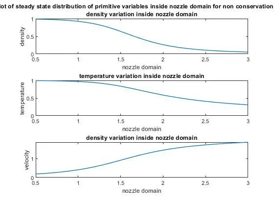
Plot for nonconservative form:

1. Plot of steady state distribution of primitive variables
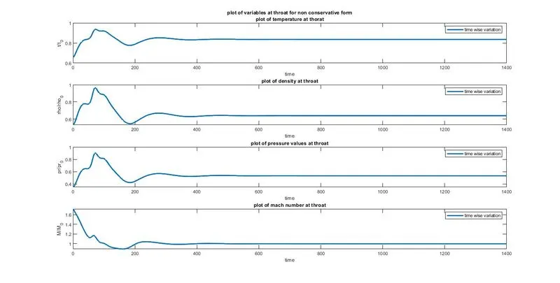
2. Plot of time wise variation of primitive variables at throat .
3. Plot of mass flow rate at different time step

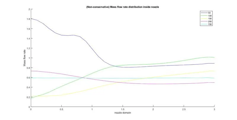
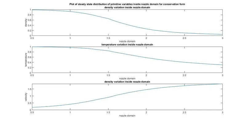
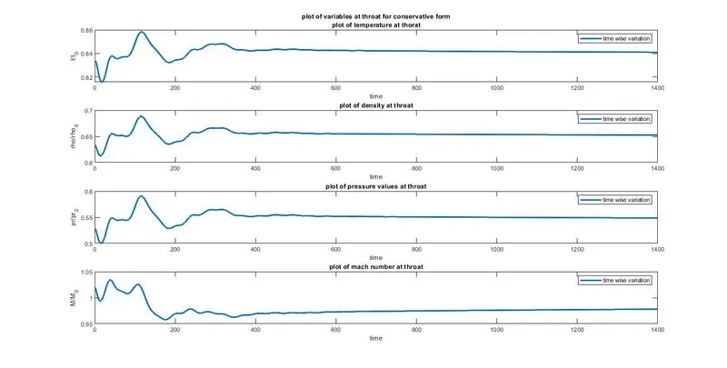
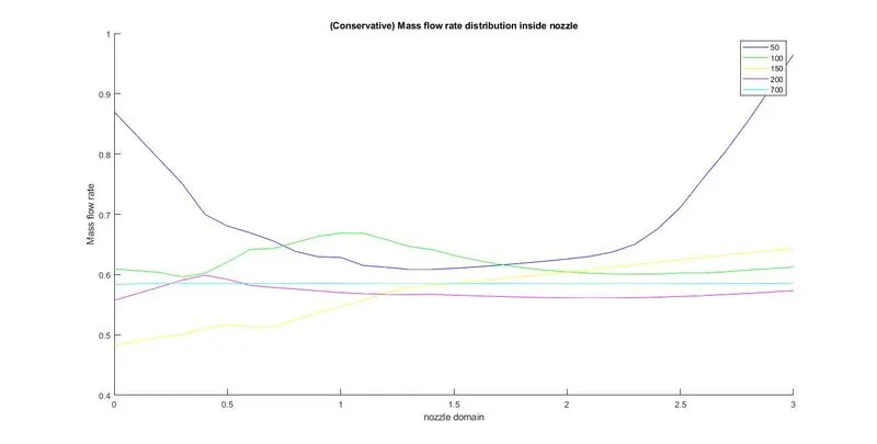
Plot for conservative form of governing equation: All the plots are similar to results obtained from analytical solution.

1. Plot of steady state distribution of primitive variables.
2. Plot of time wise variation of primitive variables at throat.
3. Plot of mass flow rate at different time step.

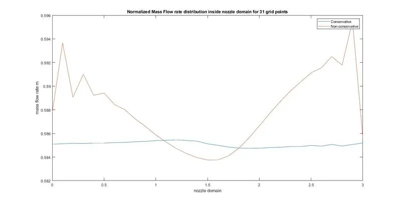
Comparison of normalized mass flow rate for both forms of governing equations:

Grid independence test on the solution :

The matter of grid independence is a serieous consideration in CFD. In general, when we solve a problem using CFD, we are emplyoing a fininte number of grid points. If everything goes well we get some numbers out for the flow filed variables at these grid points.

Assume two cases:

n = 31 & n = 61

Here we are doubling the number grids.

Now comparing the steady state solution for primitive variables at nozzle throat as shown in table below: Comparing for non-conservative solution

	`rho^star/rho^o`	`T^star/T^o`	`P^star/P^o`	`M`
n = 31	0.639	0.836	0.534	0.994
n = 61	0.638	0.835	0.533	1
Exact solution	0.634	0.833	0.528	1

Here we can see that although doubling the number of grid points did improve the numerical solution, it did so only marginally. The same is true for all location inside the nozzle. Therefore we can conclude that our original calculations using 31 grid points is essentially grid independent.

Simulation time to obtain steady state solution:

grid points	form of gov equation	time taken
n = 31	conservative	3.191 sec
n = 31	non conservative	5.1285 sec
n = 61	conservative	2.336 sec
n = 61	non conservative	3.459 sec

Conclusion

• From the table of simulation time we can conclude the simulation time to obtain steady state solution of primitive variables is less for conservative form in comparison to non conservative form
• From the grid independence test we can conclude that the original solution with 31 grid points is grid independent. We can also observe that non conservative form provide better accuracy for primitive variables.
• From the normalized mass flow rate graph comparison we can observe that mass flow rate for conservative form is more stable and hence accurate in comparison to non conservative form. But in general non conservative form is considered more accurate.