Week 9 - FVM Literature Review

FINITE VOLUME METHOD
The Finite Volume Method (FVM) is a very versatile discretization technique used in CFD. In FDM, discretization is based on dividing the domain into discrete points (greater the number of points, smaller the gridsize hence greater the accuracy), whereas FVM is based on the control volume formation of analytical fluid dynamics, where the primary step is to divide the domain into a number of control volumes (or cells) such that the variables of the interest is situated at the centroids of control volumes.
FVM is the ideal method for computing solutions with discontinuities arising in compressible flows. The most significant advantage of using FVM is that it only needs to do flux evaluations for the cell boundaries. Also, this is true for non-linear issues as well, which in turn, makes it an excellent choice for handling (non-linear) conservation laws as well. Mostly suitable for problems involving heat transfer, structural mechanics and vibrational analysis.

DIFFERNCES BETWEEN FDM & FVM:

Finite Difference Method	Finite Volume Method
Domain is disretized into number of discrete points called nodes.	Domain is discretized into a number of small elements (or cells) of geometrically simple shape.
Properties are calculated for each node individually.	Properties represented at the centroid are the average of all the points in the cell.
FDM can be used efficiently only for structured mesh.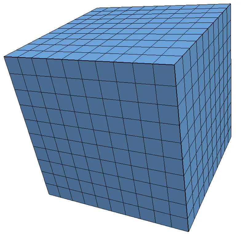	FVM can be used for unstructured mesh also.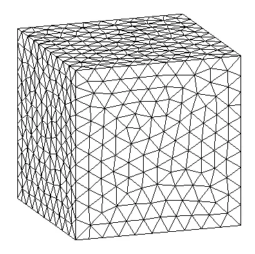
Cannot efficiently handle discontinuities in the geometry.	Suitable to handle discontinuities in the geometry.
Differential form of PDEs are used.	Integral form of PDEs are used.
Primarily uses Taylor Series.	Primarily uses Gauss-Divergence Theorem.
Extending to higher order for more accuracy is simpler.	Extending to higher order for more accuracy is much more complex.
Can be used only for linear forms of conservation laws.	Can also be used for non-linear forms of conservation laws.

INTERPOLATION SCHEMES & FLUX LIMITERS IN FVM:
Consider a 1D Steady State Heat Conduction equation with a source term.
`del/(delx)(alpha(delT)/(delx)) + S = 0`
To represent the Finite Volume approach for the above equation, we can consider this figure where P - centroid representing under consideration, L - centroid of the cell to the left, R - centroid of the cell to the right and l and r are the cell boundaries respectively.

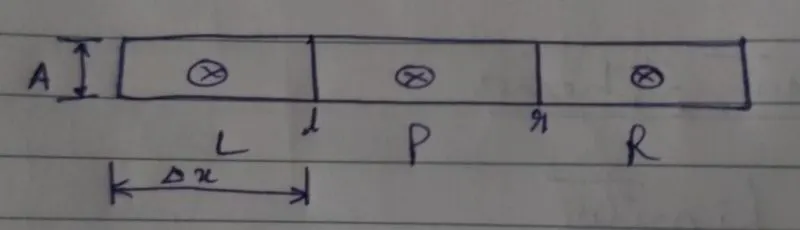
With respect to the above figure, we can now rewrite the 1D Steady State Heat Conduction equation as required for Finite Volume approach: `int_l ^r (del/(delx)(alpha(delT)/(delx)) + S)dV = 0`.
`=> int_l ^r del/(delx)(alpha(delT)/(delx))Adx + int_l^rSdV =0`
`=> [alphaA(delT)/(delx)]_l^r + overlineSdV = 0`
`=> alpha_rA(delT)/(delx_r) - alpha_lA(delT)/(delx_l) + overlineSdV = 0`
`=> alpha_rA[(T_r - T_p)/(trianglex)] - alpha_lA[(T_p - T_l)/(trianglex)] + overlineSdV = 0`
At this point, linearisation has to be performed for the source term `S` and the coefficient `alpha` since they are both functions of temperature and hence are subject to change as temperature changes.

Interpolation Schemes are methods of mathematical approximations required to compute the values at the cell surfaces. These schemes are used to transform cell centre quantities to face centres. This operation is used for many of the FVM calculations such as Gradient, Divergence and Laplacian terms. There are many types of Interpolation Schemes, we can broadly classify them into four categories:

1) Centred Schemes
a) Linear Interpolation Scheme
b) Cubic Scheme
c) Linear Interpolation with Symmetric Weighing Scheme

2) Upwinded Convection Schemes
a) Upwind Differencing Scheme
b) Linear Upwind Differencing Scheme
c) Linear with Skewness Correction Scheme
d) Linear with Filtering for High-Frequency Ringing Scheme

3) TVD Schemes
a) Limited Linear Differencing Scheme
b) Van Leer Limiter Scheme
c) MUSCL Scheme
d) Cubic Limiter Scheme

4) NVD Schemes
a) Self-Filtered Central Differencing Scheme
b) Gamma Differencing Scheme

Flux Limiters or slope limiters are basically mathematical expressions that have the effect of limiting the solution gradient near shocks and discontinuities. If the limiter acts on system fluxes, then it is known as flux limiter and if the limiter acts on system states, then it is known as slope limiter.
They are used in high resolution schemes such as MUSCL scheme, to avoid spurious oscillations (wiggles) that would otherwise occur with higher order spatial discretization schemes to shocks, discontinuities or sharp changes in the solution domain. Use of Flux Limiters, with an appropriate high resolution scheme helps us attain a TVD (Total Variation Diminishing) Solution.
The main idea behind a Flux Limiter is to limit the spatial derivatives to realistic values. For scientific and engineering porblems this is to say physically meaningful values. They are used in high resolution schemes for solving problems describes by PDEs and only come into use when sharp waves or discontinuities are present. For smoothly changing waves, the flux limiters do not operate and the spatial derivatives can be represented by higher order approximations without introducing spurious oscillation.
Mathematically, this can be explained with an example taking a 1D semi-discrete scheme for simplicity:
`(du_i)/(dt) + 1/(trianglex_i)[F(u_(i+1/2)) - F(u_(i-1/2))] = 0`
where `F(u_(i+1/2))` and `F(u_(i-1/2))` represent edge fluxes for the ith cell. If these edge fluxes can be represented by high and low resolution schemes, then a flux limiter can switch between these schemes depending upon the gradients close to that particular cell.
`F(u_(i+1/2)) = f_(i+1/2)^(low) - phi(r_i)(f_(i+1/2)^(low)-f_(i+1/2)^(high))`
`F(u_(i-1/2)) = f_(i-1/2)^(low) - phi(r_(i-1))(f_(i-1/2)^(low)-f_(i-1/2)^(high))`where `f^(low)`, `f^(high)` are the low and high resolution schemes respectively and `phi(r)` is the flux limiter function, `r` representing the ratio of successive gradients on the solution mesh, i.e. `r = (u_i - u_(i-1))/(u_(i+1) - u_i)`.
The limiter function is constrained to be greater than or equal to zero, `phi(r) >= 0`. Hence, limiter equals to zero implies sharp gradient, opposite slopes or zero gradient and the flux is represented by a low resolution scheme. Similarly, when the limiter equals 1 (smooth solution), it is represented by a high resolution scheme. Different limiters have different switching characteristics and no one limiter works well for all problems. Therefore, a particular limiter has to be chosen based on the type of problem and the solution scheme in a trial and error basis.