Week 5.1 - Mid term project - Solving the steady and unsteady 2D heat conduction problem
AIM:
1) To solve 2D Steady State Heat Conduction Equation using implicit approach with point iterative techniques - Jacobi, Gauss Seidel and SOR methods.
2) To solve 2D Unsteady State Heat Conduction Equation using explicit approach.
3) To solve 2D Unsteady State Heat Conduction Equation using implicit approach with point iterative techniques - Jacobi, Gauss Seidel and SOR methods.
GIVEN DATA:
1) Top Boundary = 600K
2) Bottom Boundary = 900K
3) Left Boundary = 400K
4) Right Boundary = 800K
5) Absolute Error Tolerance = 1e-4
ASSUMPTIONS:
1) Assume a square domain of length 1 unit.
2) Assume number of nodes along X axis is equal to number of nodes along Y axis which is equal to 10.
3) Assume Temperature at the corners is average of the two boundary values.
4) Assume `omega = 1.1` initially for SOR technique.
5) Assume initial temperature 300K (ambient temperature) across the domain.
GOVERNING EQUATION: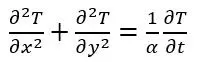
The above equation is the 2-Dimensional Heat Conduction Equation, where `alpha` is the thermal diffusivity.
STEADY STATE HEAT CONDUCTION:
In steady state, the 2D Heat Conduction Equation gets reduced to 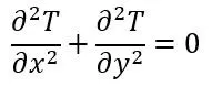
Here, it is seen that RHS is equated to zero, this is because in steady state the temperature differential with respect to time is zero. After discretization and rearranging of the terms, the equation shown above gets transformed to 
CODE:
The given data, the assumed values and the constants required are all defined appropriately so as to have the variables ready for iteration loop. The user chooses the iterative method by entering the correct numerical value - 1 for Jacobi, 2 for Gauss Seidel and 3 for SOR. Here, SOR technique is performed over Gauss Seidel scheme. This choice is made available to the user by the use of an if-elseif ladder. Here since the problem involves two dimensions, two for loops are used, one nested in the other, for spatial loops. The iterative loop runs until the absolute error value is lesser than the tolerance value specified. Also, the value of `omega` is varied with each trial so as to obtain minimum number of iterations in SOR method, it is observed that for `omega = 1.1` we get no. of iterations = 92 which reduces to 28 when `omega = 1.5` beyond which the value overshoots and the no. of iterations increases again. Finally, the temperature distribution is plotted as shown below with the help of 'contourf' command with the help of a colorbar.
%2D Steady State Heat Conduction Equation
%Temperature Distribution in Steady State Heat Conduction
clear all
close all
clc
%Discretization & Domain Length
n = 10; %no. of nodes
L = 1; %length of the domain
%defining X and Y in discretization plane
x = linspace(0, L, n);
y = linspace(0, L, n);
dx = abs(x(1) - x(2));
dy = abs(y(1) - y(2));
%defining temperature value throughout discretization plane with ambient temperature 300K
T = 300*ones(n, n);
%initial boundary conditions
T(1:end, 1) = 400; %left
T(1:end, end) = 800; %right
T(1, 1:end) = 600; %top
T(end, 1:end) = 900; %bottom
%average values for T at corners of discretization plane
T(1, 1) = 500; %top-left (400+600)/2
T(1, end) = 700; %top-right (600+800)/2
T(end, 1) = 650; %bottom-left (400+900)/2
T(end, end) = 850; %bottom-right (800+900)/2
%intialising zeroth iteration value
Told = T;
%constant values
k = (2*(dx^2+dy^2)/((dx^2)*(dy^2)));
w = 1.1; %omega value for SOR method
error = 100;
tol = 1e-4;
iteration = 0;
method = input('Enter (1) for Jacobi, (2) for Gauss_Siedel and (3) for SOR method: ');
if method == 1
    while(error>tol)
        for i = 2:(n-1)
            for j = 2:(n-1)
                H = (Told(i-1, j) + Told(i+1, j))/dx^2;
                V = (Told(i, j-1) + Told(i, j+1))/dy^2;
                T(i, j) = (H + V)/k;
            end
        end
        error = max(max(abs(Told - T))); %computing error value
        Told = T; %updating Told array after spatial loop
        iteration = iteration + 1; %updating Iteration count
    end
elseif method == 2
        while(error>tol)
            for i = 2:n-1
                for j = 2:n-1
                    H = (T(i-1, j) + T(i+1, j))/dx^2;
                    V = (T(i, j-1) + T(i, j+1))/dy^2;
                    T(i, j) = (H + V)/k;
                end
            end
            error = max(max(abs(Told - T))); %computing error value
            Told = T; %updating Told array after spatial loop
            iteration = iteration + 1; %updating Iteration count
        end
elseif method == 3 %SOR method is done over Gauss Seidel method
        while(error>tol)
            for i = 2:n-1
                for j = 2:n-1
                    H = (T(i-1, j) + T(i+1, j))/dx^2;
                    V = (T(i, j-1) + T(i, j+1))/dy^2;
                    T(i, j) = ((1 - w) * Told(i, j)) + (w * (H + V)/k);
                end
            end
            error = max(max(abs(Told - T))); %computing error value
            Told = T; %updating Told array after spatial loop
            iteration = iteration + 1; %updating Iteration count
        end
else
    disp('Invalid Input')
    return
end
%plotting
figure(1)
contourf(x, y, T)
clabel(contourf(x, y, T))
colorbar
colormap(jet)
set(gca, 'ydir', 'reverse')
title(sprintf('Total no. of Iterations = %d', iteration));
GRAPHS:
1) 2D Steady State Heat Conduction - Jacobi Scheme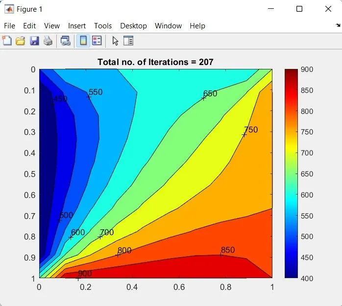
2) 2D Steady State Heat Conduction - Gauss Seidel Scheme 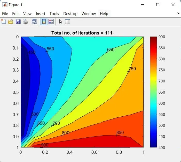
3) 2D Steady State Heat Conduction - SOR Scheme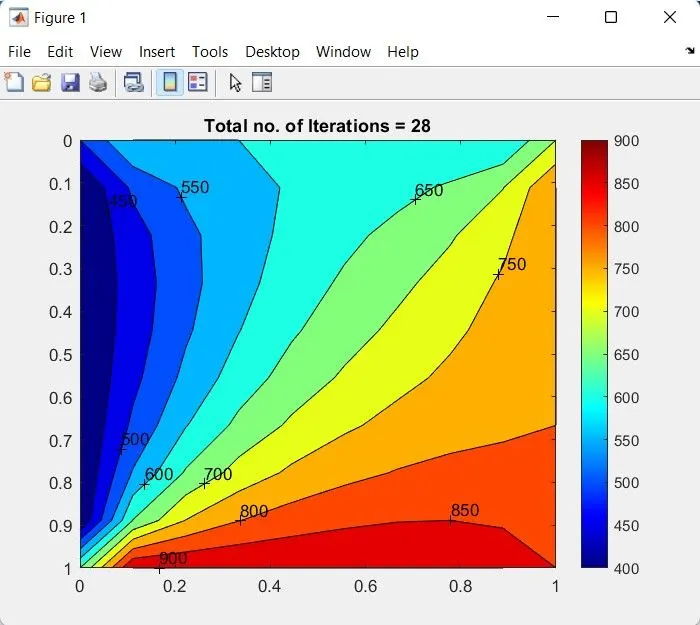
2D UNSTEADY / TRANSIENT HEAT CONDUCTION EQUATION:
The above equation represents 2D Unsteady / Transient Heat Conduction. This equation can be solved by use of two approaches – explicit and implicit.
After discretization, for explicit approach the terms are rearranged and the equation can be written as follows
After discretization, for implicit approach the terms are rearranged and the equation can be written as follows
CODE:
The given data, the assumed values and the constants required are all defined appropriately so as to have the variables ready for iteration loop. The user chooses the iterative method by entering the correct numerical value - 1 for Explicit Approach, 2 for Implicit Approach Jacobi Scheme, 3 for Implicit Approach Gauss-Seidel Scheme and 4 for Implicit Approach SOR Scheme. Here, SOR technique is performed over Gauss-Seidel scheme. This choice is made available to the user by the use of an if-elseif ladder. Here since the problem involves two dimensions, two for loops are used, one nested in the other, for spatial loops. The iterative loop runs until the absolute error value is lesser than the tolerance value specified. These loops are nested in another while loop called Time Loop, which runs until the convergence value is lesser than the tolerance value. Finally, the temperature distribution is plotted as shown below with the help of 'contourf' command with the help of a colorbar.
%2D Unsteady State Heat Conduction Equation
%Temperature Distribution in Unsteady State Heat Conduction
clear all
close all
clc
%Discretization & Domain Length
n = 10; %no. of nodes
L = 1; %length of the domain
dt = 5e-3;
%defining X and Y in discretization plane
x = linspace(0, L, n);
y = linspace(0, L, n);
dx = abs(x(1) - x(2));
dy = abs(y(1) - y(2));
%defining temperature value throughout discretization plane with ambient temperature 300K
T = 300*ones(n, n);
%initial boundary conditions
T(1:end, 1) = 400; %left
T(1:end, end) = 800; %right
T(1, 1:end) = 600; %top
T(end, 1:end) = 900; %bottom
%average values for T at corners of discretization plane
T(1, 1) = 500; %top-left (400+600)/2
T(1, end) = 700; %top-right (600+800)/2
T(end, 1) = 650; %bottom-left (400+900)/2
T(end, end) = 850; %bottom-right (800+900)/2
%intialising zeroth iteration value
Told = T;
%intialising array for previous timestep
Tprev = T;
%Initialising convergence array for time loop condition
convergence = 100;
%constant values
w = 1.1; %omega value for SOR method
a = 0.6; %thermal diffusivity alpha
k1 = (a*dt)/(dx^2);
k2 = (a*dt)/(dy^2);
CFL = k1 + k2;
error = 100;
tol = 1e-4;
iteration = 0; % to keep count of iterations in implicit methods
count = 0; % to keep count of time loops in explicit method
method = input('Enter (1) for Explicit approach, (2) for Implicit-Jacobi approach, (3) for Implicit-Gauss_Seidel approach and (4) for Implicit_SOR approach: ');
if method == 1 %Explicit Approach
    while(convergence>tol)
            for i = 2:n-1
                for j = 2:n-1
                    term1 = k1*(Tprev(i-1, j) - 2*Tprev(i, j) + Tprev(i+1, j));
                    term2 = k2*(Tprev(i, j-1) - 2*Tprev(i, j) + Tprev(i, j+1));
                    T(i, j) = Tprev(i, j) + term1 + term2;
                end
            end
        convergence = max(max(abs(Tprev-T))); %computing convergence value after each time loop
        residual(count+1) = convergence;
        Tprev = T; %Updating Tprev array after time loop
        count = count + 1; % Updating Time loop count
        %plotting
        figure(1)
        contourf(x, y, T)
        clabel(contourf(x, y, T))
        colorbar
        colormap(jet)
        set(gca, 'ydir', 'reverse')
        title(sprintf('Total no. of Explicit Time Loops = %d', count))
    end
elseif method == 2 %Jacobi Scheme
    while(convergence>tol)
        while(error>tol)
            for i = 2:n-1
                for j = 2:n-1
                    term4 = 1/(1 + 2*k1 + 2*k2);
                    term5 = k1/(1 + 2*k1 + 2*k2);
                    term6 = k2/(1 + 2*k1 + 2*k2);
                    H = Told(i-1, j) + Told(i+1, j);
                    V = Told(i, j-1) + Told(i, j+1);
                    T(i, j) = (term4*Tprev(i, j)) + (term5*H) +(term6*V);
                end
            end
            error = max(max(abs(Told-T))); %computing error value after each spatial loop
            Told = T; %Updating Told array after spatial loop
            iteration = iteration + 1; % Updating iteration count
        end
        error = 100;
        convergence = max(max(abs(Tprev-T))); %computing convergence value after each time loop
        Tprev = T; %Updating Tprev array after time loop
        %plotting
        figure(1)
        contourf(x, y, T)
        clabel(contourf(x, y, T))
        colorbar
        colormap(jet)
        set(gca, 'ydir', 'reverse')
        title(sprintf('Total no. of Jacobi Iterations = %d', iteration))
    end
elseif method == 3 %Gauss-Seidel Scheme
    while(convergence>tol)
        while(error>tol)
            for i = 2:n-1
                for j = 2:n-1
                    term4 = 1/(1 + 2*k1 + 2*k2);
                    term5 = k1/(1 + 2*k1 + 2*k2);
                    term6 = k2/(1 + 2*k1 + 2*k2);
                    H = T(i-1, j) + T(i+1, j);
                    V = T(i, j-1) + T(i, j+1);
                    T(i, j) = (term4*Tprev(i, j)) + (term5*H) +(term6*V);
                end
            end
            error = max(max(abs(Told-T))); %computing error value after each spatial loop
            Told = T; %Updating Told array after spatial loop
            iteration = iteration + 1; % Updating iteration count
        end
        error = 100;
        convergence = max(max(abs(Tprev-T))); %computing convergence value after each time loop
        Tprev = T; %Updating Tprev array after time loop
        %plotting
        figure(1)
        contourf(x, y, T)
        clabel(contourf(x, y, T))
        colorbar
        colormap(jet)
        set(gca, 'ydir', 'reverse')
        title(sprintf('Total no. of Gauss-Seidel Iterations = %d', iteration))
    end
elseif method == 4 %SOR Scheme
    while(convergence>tol)
        while(error>tol)
            for i = 2:n-1
                for j = 2:n-1
                    term4 = 1/(1 + 2*k1 + 2*k2);
                    term5 = k1/(1 + 2*k1 + 2*k2);
                    term6 = k2/(1 + 2*k1 + 2*k2);
                    H = T(i-1, j) + T(i+1, j);
                    V = T(i, j-1) + T(i, j+1);
                    T(i, j) = ((1 - w)*Told(i, j)) + (w*((term4*Tprev(i, j)) + (term5*H) +(term6*V)));
                end
            end
            error = max(max(abs(Told-T))); %computing error value after each spatial loop
            Told = T; %Updating Told array after spatial loop
            iteration = iteration + 1; % Updating iteration count
        end
        error = 100;
        convergence = max(max(abs(Tprev-T))); %computing convergence value after each time loop
        Tprev = T; %Updating Tprev array after time loop
        %plotting
        figure(1)
        contourf(x, y, T)
        clabel(contourf(x, y, T))
        colorbar
        colormap(jet)
        set(gca, 'ydir', 'reverse')
        title(sprintf('Total no. of SOR Iterations = %d', iteration))
    end
else
    disp('Invalid Input')
    return
end
GRAPHS:
1) 2D Unsteady State Heat Conduction - Explicit Approach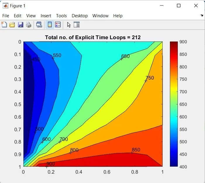
2) 2D Unsteady State Heat Conduction - Implicit Approach - Jacobi Scheme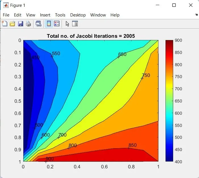
3) 2D Unsteady State Heat Conduction - Implicit Approach - Gauss-Seidel Scheme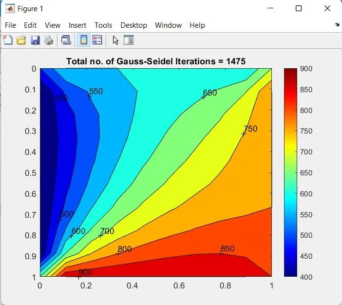
4) 2D Unsteady State Heat Conduction - Implicit Approach - SOR Scheme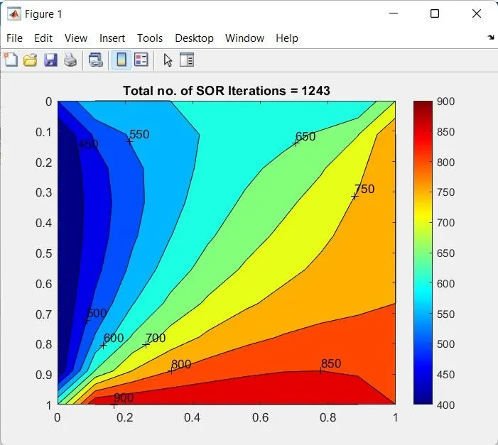
INFERENCES:
From the outputs generated and the graphs plotted we can observe the number of iterations for each scheme decrease in the following order: Jacobi > Gauss Seidel > SOR. Here, we also learn that `omega` value plays an important role in SOR technique. Also, for explicit approach we learn that CFL = k1 + k2 must be lesser than 0.5 to attain proper results. To obtain required CFL value, we must change the values of a (thermal diffusivity alpha) and dt (time step) values.