Week 11 - Simulation of Flow through a pipe in OpenFoam
AIM:
1) To simulate an axi-symmetric flow by applying a wedge boundary condition.
2) Validate the results with Hagen-Poiseuille's equation for fully developed flow.
3) Validate the Hydro-dynamic length with numerical result.
4) Validate the fully developed flow velocity profile with analytical velocity profile.
5) Validate the maximum velocity and pressure drop for fully developed flow.
6) Post-process shear stress and validate wall shear stress for fully developed flow.
DATA:
1) Flow is laminar.
2) Reynold's Number `R_e = 2100`.
3) Wedge angle `theta = 5`.
4) Pipe radius `r = 0.01m`.
5) Pipe length `L = 2.5m`
6) Pipe axis is along X-axis.
7) Kinematic Viscosity of water at 300K `nu = 8.55*10^-7 m^2/s`
8) Density of water at 300K `rho = 996.59 (kg)/m^3`
9) Dynamic Viscosity at 300K `mu = 8.52*10^-4 Pa*s`
GOVERNING EQUATIONS:
Hydrodynamic Entry Length `((L_(hy))/(d))_(l) = 0.05R_e`.
`=> L_(hy) = 0.05*2100*0.02`
`=> L_(hy) = 2.1m`
Hence we assume the total length of the pipe to be 2.5m (with 0.4m of fully developed flow).
Hagen Poiseuille Equations
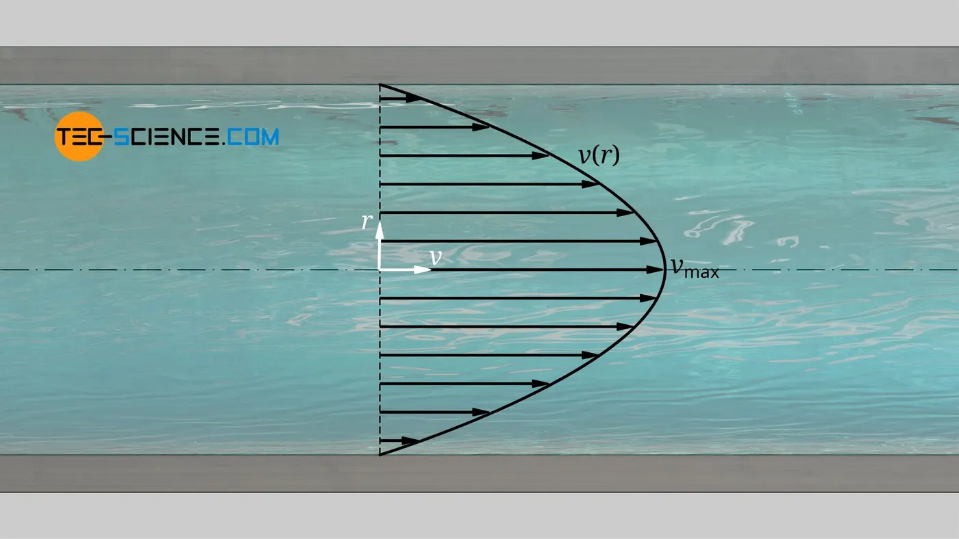
Velocity`=> v(r) = -R^2/(4mu)(dp)/(dx)*[1-(r/R)^2]`
Maximum Velocity `=> v_(max) = -R^2/(4mu) (dp)/(dx)`
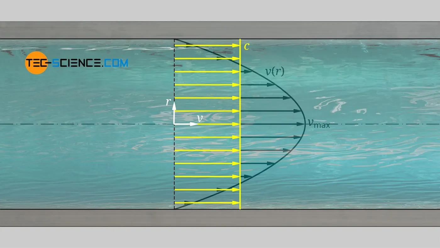
Pressure loss `=> trianglep_l = (8mu*triangleL)/(R^2)*v_(avg)`
where `v_(avg)` represents mean flow velocity `V_(avg) = 1/2 * v_(max)`
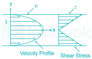
Shear Stress `=> tau = mu*(dv(r))/(dr)`
ANALYTICAL CALCULATIONS:
Velocity -
`R_e = (rhovD)/(mu) = (vD)/(nu)`
Here pipe diameter is used rather than calculating the characteristic length as we are considering a long pipe in the current simulation.
`v_(avg) = (R_enu)/(D) = (2100*8.55*10^-7)/(0.02)`
`therefore v_(avg) = 0.08976m/s`
Maximum Velocity -
`=> v_(max) = 2 * v_(avg) `
`therefore v_(max) = 0.1795 m/s`
Pressure Drop -
As per Hagen Poiseuille Equations,
`triangleP = (32*mu*L*v_(avg))/(D^2)`
`=> triangleP = (32*8.52*10^-4*3.04*0.0155)/(0.02^2)`
`therefore triangleP = 58.90Pa`
Kinetic Pressure -
`P_k = (P_s)/rho`
`=> P_k = 15.2951/996.59`
`therefore P_k = 0.01535 m^2/s^2`
PROCEDURE:
The given problem statement involves axi-symmetric, laminar flow through a constant cross-section pipe following Hagen-Poiseuille's equations and for this a suitable tutorial is selected from the FOAM_TUTORIALS folder. Similar to our problem is the "cavity" tutorial in the folder "incompressible" under the solver "icoFoam". We first copy this folder to the FOAM_RUN folder using the command "cp -r" in the command line terminal.
Now that we have the most relevant case-setup "cavity" copies ot the FOAM_RUN folder, we can start editing it to match our problem statement more accurately. Initially, we edit the the file "blockMeshDict" in the system folder to attain geometry similar to our case.
blockMeshDict file:
/*--------------------------------*- C++ -*----------------------------------*
  =========             	|
  \  	  /  F ield     	| OpenFOAM: The Open Source CFD Toolbox
   \	 /   O peration 	| Website:  https://openfoam.org
    \  /     A nd       	| Version:  9
     \/      M anipulation      |
*---------------------------------------------------------------------------*/
FoamFile
{
	format  	ascii;
	class   	dictionary;
	object  	blockMeshDict;
}
// * * * * * * * * * * * * * * * * * * * * * * * * * * * * * * * * * * * * * //

convertToMeters 1;


// Mesh metrics

nx 50;
ny 1;
nz 100;

grad (1 1 1);


/*


 v2--------v1-------v5-------v4
  \  	  /          \      /
   \	 /            \    /
    \   /              \  /
     \ /                \/
      v0-----------------v3


*/


theta 2.5; //(wedge angle)/2 => 5/2=2.5
r 0.01;
L #calc "(0.05*2100*2*$r) + 0.4";
// L=Lhy+0.4=2.5
//0.05*Re*D = Lhy

sinTheta #calc "$r*sin(degToRad($theta))";
msinTheta #calc "-1.0*$sinTheta";
cosTheta #calc "$r*cos(degToRad($theta))";


vertices
(
	(0 0 0)               	//point 0
	(0 $cosTheta $msinTheta)  //point 1
	(0 $cosTheta $sinTheta)   //point 2
	($L 0 0)              	//point 3
	($L $cosTheta $msinTheta) //point 4
	($L $cosTheta $sinTheta)  //point 5
);

blocks
(
	hex (0 1 2 0 3 4 5 3) ($nx $ny $nz) simpleGrading ($grad)
);

edges
(
);

boundary
(
	inlet
	{
    	type patch;
    	faces
    	(
        	(0 1 2 0)
    	);
	}
	left
	{
    	type wedge;
    	faces
    	(
        	(0 2 5 3)
    	);
	}
	right
	{
    	type wedge;
    	faces
    	(
        	(0 3 4 1)
    	);
	}
	outlet
	{
    	type patch;
    	faces
    	(
        	(3 5 4 3)
    	);
	}
	top
	{
   	 type wall;
   	 faces
   	 (
   		 (1 4 5 2)
   	 );
	}
);

mergePatchPairs
(
);

// ************************************************************************* //
After editing the blockMeshDict file to attain the required geometry, we run the "blockMesh" command in the command terminal. Thereupon the paraFoam command in run for post-processing, this creates the cavity. OpenFOAM which can be viewed and analysed in ParaView. After checking the mesh quality, we come back to the cavity folder and edit the files U and p in the 0 folder. These files signify the initial states for velocity & pressure and here we edit these files to attain the initial states pertinent to our problem statement.
Velocity Initial State file - U:
/*--------------------------------*- C++ -*----------------------------------*
  =========             	|
  \  	  /  F ield     	| OpenFOAM: The Open Source CFD Toolbox
   \	 /   O peration 	| Website:  https://openfoam.org
    \  /     A nd       	| Version:  9
     \/      M anipulation      |
*---------------------------------------------------------------------------*/
FoamFile
{
	format  	ascii;
	class   	volVectorField;
	object  	U;
}
// * * * * * * * * * * * * * * * * * * * * * * * * * * * * * * * * * * * * * //

dimensions  	[0 1 -1 0 0 0 0];

internalField   uniform (0 0 0);

boundaryField
{
	inlet
	{
    	type        	fixedValue;
    	value       	uniform (0.08976 0 0);
	}

	left
	{
    	type        	wedge;
	}

	right
	{
    	type        	wedge;
	}

	top
	{
    	type        	noSlip;
	}

	outlet
	{
    	type        	zeroGradient;
	}
}

// ************************************************************************* //
Pressure Initial State file - p:
/*--------------------------------*- C++ -*----------------------------------*
  =========             	|
  \  	  /  F ield     	| OpenFOAM: The Open Source CFD Toolbox
   \	 /   O peration 	| Website:  https://openfoam.org
    \  /     A nd       	| Version:  9
     \/      M anipulation      |
*---------------------------------------------------------------------------*/
FoamFile
{
	format  	ascii;
	class   	volScalarField;
	object  	p;
}
// * * * * * * * * * * * * * * * * * * * * * * * * * * * * * * * * * * * * * //

dimensions  	[0 2 -2 0 0 0 0];

internalField   uniform 0;

boundaryField
{
	inlet
	{
    	type        	zeroGradient;
	}

	left
	{
    	type        	wedge;
	}

	right
	{
    	type        	wedge;
	}

	top
	{
    	type        	zeroGradient;
	}

	outlet
	{
    	type        	fixedValue;
    	value    	uniform 0;
	}
}

// ************************************************************************* //
In this file, the pressure is pressure values are specified in terms of kinetic pressure (`P_k`).
Also before the solver is run we have to check the relevant transport property (kinematic diffusivity `nu`) in the file "transportProperties" located in the folder "constants".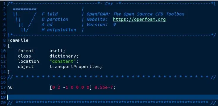
After the initial states are well-defined with respect to our problem statement and the meshing subscribed over the geometry is checked.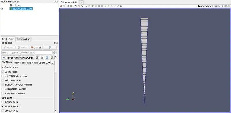
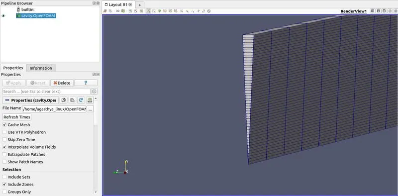
Then we run the icoFoam solver by using the "icoFoam" command in the command line terminal. Once the icoFoam solver is run we can observe the simulation in ParaView and analyse the results. Once the simulation is complete, the variations in pressure are checked throughout the geometry, at the inlet and at the outlet: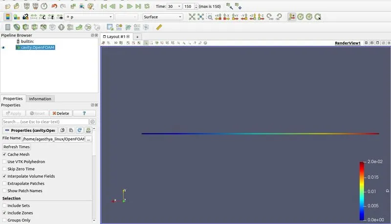
Similarly, the velocity profile is checked throughout the geometry, at the inlet and at the outlet: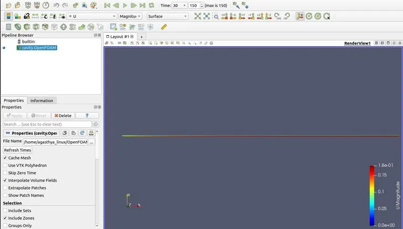
To further analyse the velocity profile, we use the plot over line command in ParaView to observe the velocity profiles at specific cross-sections in the geometry.
Velocity Profile at 0.01m from the inlet: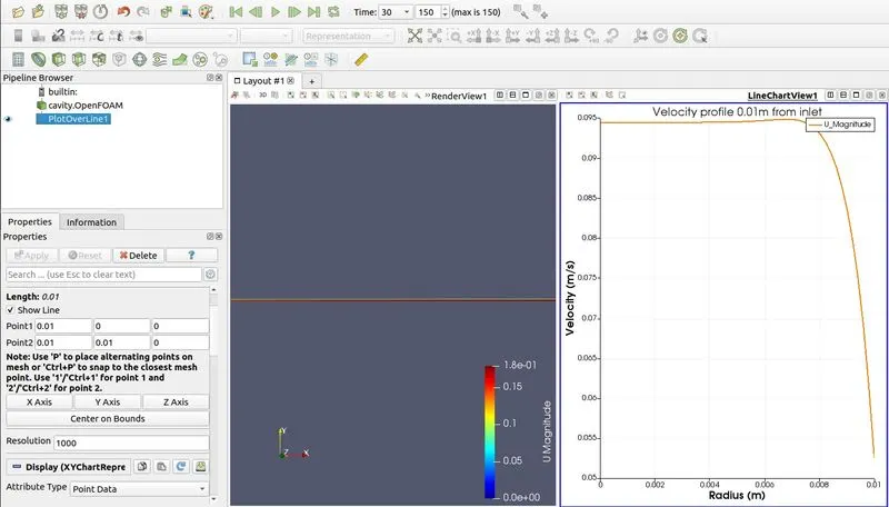
Velocity Profile at 1m from the inlet: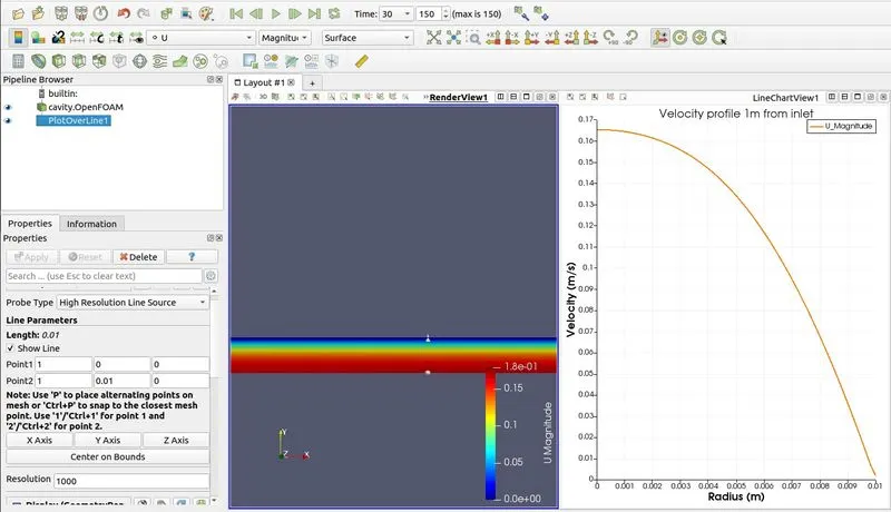
Velocity Profile at 2m from the inlet: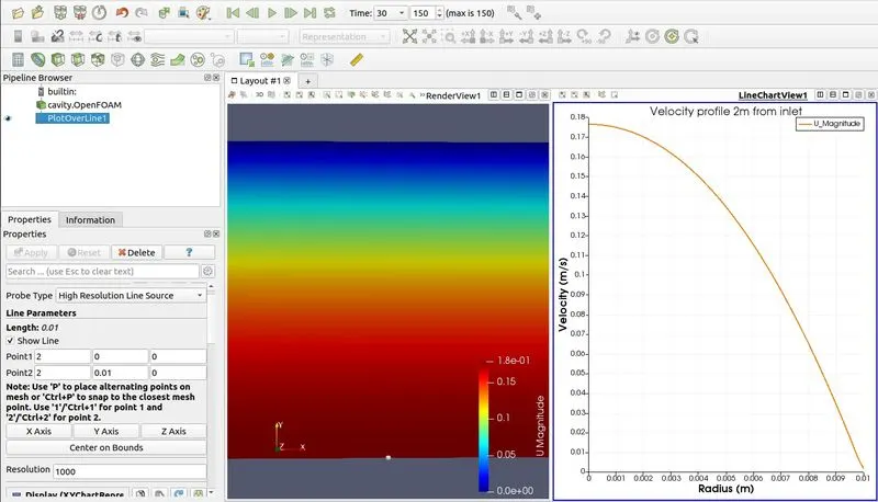
Velocity Profile at 2.11m from the inlet: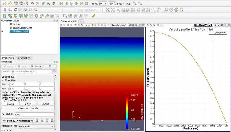
Velocity Profile at 2.5m from the inlet: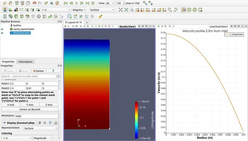
Also, with the use of Hagen Poiseuille Equation, we can also analyse the shear stress in the pipe caused due to the laminar flow: 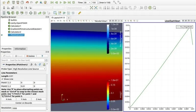
To further make sense of these results, we compare them to the results obtained in the analytical calculations performed previously. We observe that after flow passes through hydrodynamic entry length, velocity profile is fully developed. This can be observed in the velocity profile 2.11m from inlet (2.11 > 2.1 where 2.1m is hydrodynamic entry length).
INFERENCES:
Thus, by observing the specimen graphs and by comparing them with the graphs plotted in ParaView, we can say that the wedge simulation has been successful and the parameters have been properly defined and plotted across the radius of the sector i.e. from r=0 to r=0.01m, as per Hagen Poiseuille Equations. And by observing th egraphs obtained in ParaView, we can say that when r=0 i.e. at the centre there will be zero shear stress and maximum velocity. On the other hand, at r=0.01m i.e. at the circumference shear stress will be maximum and velocity will be zero.