Week 7 - Simulation of a 1D Super-sonic nozzle flow simulation using Macormack Method

AIM:
1) To simulate isentropic flow through subsonic-supersonic nozzle using MacCormack Method using both Conservative and Non-Conservative forms of the governing equations.
2) To determine steady state distribution of flow-field variables inside the nozzle.
3) To perform Grid Independence test on the simulation.
4) To plot the time-wise variation of the primitive variables.
5) To show the flow rate of mass flow distribution inside the nozzle at different time-steps.
6) To compare the normalised mass flow rate distributions attained using both forms of the governing equations.

GOVERNING EQUATIONS:
Non-Dimensional Governing Equations in Non-Conservative Form:-
Continuity Equation -
`(delrho')/(delt') = - rho'(delv')/(delx') - rho'v'(del(ln A'))/(delx') - v'(delrho')/(delx')'`
Momentum Equation -
`(delv')/(delt') = -v'(delv')/(delx') - 1/gamma((delT')/(delx') + (T')/(rho')(delrho')/(delx'))`
Energy Equation -
`(delT')/(delt') = -v'(delT')/(delx') - (gamma - 1)T'((delv')/(delx') + v'(del(ln A'))/(delx'))`

Non-Dimensional Governing Equations in Conservative Form:-
Continuity Equation -
`(del(rho'A'))/(delt') + (del(rho'A'v'))/(delx') = 0`
Momentum Equation -
`(del(rho'A'v'))/(delt') + (del(rho'A'v'^2 + (1/gamma)rho'A'))/(delx') = (rho')/gamma(delA')/(delx')`
Energy Equation -
`(del(rho'A'((T')/(gamma-1)+(gammav'^2)/(2))))/(delt')+ (del(rho'A'v'((T')/(gamma-1)+(gammav'^2)/(2))+rho'A'v'))/(delx') = 0`
In the Conservative Form, the above non-dimensional governing equations are expressed in the terms of solutions vectors - U1, U2 and U3; flux vectors - F1, F2 and F3 and a source term J2. These terms are expressed as follows -
`U1 = rho'A'`
`U2 = rho'A'v'`
`U3 = rho'A'((T')/(gamma-1) + (gammav'^2)/(2))`
`F1 = rho'A'v'`
`F2 = rho'A'v'^2 + (rho'A')/(gamma)`
`F3 = rho'A'v'((T')/(gamma-1)+(gammav'^2)/(2)) + rho'A'v'`
`J2 = (rho')/(gamma)(delA')/(delx')`
With these terms, we can express the non-dimensional governing equations as follows -
`(delU1)/(delt') = -(delF1)/(delx')`
`(delU2)/(delt') = -(delF2)/(delx')+J2`
`(delU3)/(delt') = -(delF3)/(delx')`

PROCEDURE:
MacCormack Method:
MacCormack Method is a discretisation scheme used for the numerical solution of hyperbolic partial differential equations. This finite difference method is a time marching method using the explicit approach. It can be split into two steps - the predictor step and the corrector step. The steps for implementing the MacCormack's Method for Non-Conservative Form is as follows:
Initially, we take the initial conditions and calculate the values for the predictor step. Here we calculate the LHS terms of the governing equations - `((delf)/(delt))_p` where `f = rho, v, T`.
Once we have executed the predictor step, we perform the solution update as follows:
`f^star = f_i+((delf)/(delt))_ptrianglet`
With this new solution `f^star`, we calculate the corrector step - `((delf^star)/(delt))_c`
Next we calculate the average time derivative, i.e. the arithmetic mean of the predictor and the corrector values -
`((delf)/(delt))_(avg)=0.5[((delf)/(delt))_p + ((delf)/(delt))_c]`With this new time derivative, we find the actual functional value in the subsequent time step
`f^2 = f_i + ((delf)/(delt))_(avg)trianglet`
Also we have to take note that in the predictor step backward differencing is used and in the corrector step froward differencing is used for the discretization of the space terms.

CODE:
Main Program

%Quasi 1D Supersonic Nozzle Flow using Macormack method
clear all
close all
clc
n = 31; %Number of Nodes
x = linspace(0, 3, n); %Domain length
gamma = 1.4;
method = input('Enter (1) for Non-Conservative Form and (2) for Conservative Form: n');
if method == 1
    [x, v, T, rho, M, P, mdot, M_thrt, rho_thrt, T_thrt, P_thrt,  mdot_thrt, iteration_no, residual1, residual2, residual3] = NCF(n, x, gamma);
    %Plotting
    %figure(1)
    %plot(x, mdot_thrt(different timesteps))
    figure(2)
    %plot(x, v, x, T, x, rho, x, M, x, P, LineWidth=2)
    %legend('Velocity', 'Temperature Ratio', 'Density Ratio', 'Mach Number', 'Pressure Ratio')
    subplot(5, 1, 1)
    plot(x, M, LineWidth=2, Color='r')
    ylabel('Mach Number')
    grid on
    title('Steady State Distribution of variables inside the nozzle - Non-Conservative Form')
    subplot(5, 1, 2)
    plot(x, P, LineWidth=2, Color='g')
    ylabel('Pressure Ratio')
    grid on
    subplot(5, 1, 3)
    plot(x, T, LineWidth=2, Color='b')
    ylabel('Temperature Ratio')
    grid on
    subplot(5, 1, 4)
    plot(x, rho, LineWidth=2, Color='y')
    ylabel('Density Ratio')
    grid on
    subplot(5, 1, 5)
    plot(x, mdot, LineWidth=2, Color='m')
    xlabel('Nozzle Length')
    ylabel('Mass Flow Rate')
    grid on
    figure(3)
    plot(iteration_no, M_thrt, iteration_no, rho_thrt, iteration_no, T_thrt, iteration_no, P_thrt,  iteration_no, mdot_thrt, LineWidth=2)
    grid on
    xlabel('Number of Timesteps')
    legend('Mach Number', 'Density Ratio', 'Temperature Ratio', 'Pressure Ratio', 'Mass flow rate')
    title('Time-wise variation of variable at nozzle throat - Non-Conservative Form')
    figure(4)
    plot(iteration_no, residual1, iteration_no, residual2, iteration_no, residual3, LineWidth=2)
    grid on
    xlabel('Number of Timesteps')
    ylabel('Residuals')
    legend('Density Ratio Residuals', 'Velocity Ratio Residuals', 'Temperature Ratio Residuals')
    title('Residual Values - Non-Conservative Form')
elseif method == 2
    [x, v, T, rho, M, P, mdot, M_thrt, rho_thrt, T_thrt, P_thrt, mdot_thrt, iteration_no, residual1, residual2, residual3] = CF(n, x, gamma);
    %Plotting
    %figure(1)
    %plot(x, mdot_thrt(different timesteps))
    figure(2)
    %plot(x, v, x, T, x, rho, x, M, x, P, LineWidth=2)
    %legend('Velocity', 'Temperature Ratio', 'Density Ratio', 'Mach Number', 'Pressure Ratio')
    subplot(5, 1, 1)
    plot(x, M, LineWidth=2, Color='r')
    ylabel('Mach Number')
    grid on
    title('Steady State Distribution of variables inside the nozzle - Conservative Form')
    subplot(5, 1, 2)
    plot(x, P, LineWidth=2, Color='g')
    ylabel('Pressure Ratio')
    grid on
    subplot(5, 1, 3)
    plot(x, T, LineWidth=2, Color='b')
    ylabel('Temperature Ratio')
    grid on
    subplot(5, 1, 4)
    plot(x, rho, LineWidth=2, Color='y')
    ylabel('Density Ratio')
    grid on
    subplot(5, 1, 5)
    plot(x, mdot, LineWidth=2, Color='m')
    xlabel('Nozzle Length')
    ylabel('Mass Flow Rate')
    grid on
    figure(3)
    plot(iteration_no, M_thrt, iteration_no, rho_thrt, iteration_no, T_thrt, iteration_no, P_thrt,  iteration_no, mdot_thrt, LineWidth=2)
    grid on
    xlabel('Number of Timesteps')
    legend('Mach Number', 'Density Ratio', 'Temperature Ratio', 'Pressure Ratio', 'Mass flow rate')
    title('Time-wise variation of variable at nozzle throat - Conservative Form')
    figure(4)
    plot(iteration_no, residual1, iteration_no, residual2, iteration_no, residual3, LineWidth=2)
    grid on
    xlabel('Number of Timesteps')
    ylabel('Residuals')
    legend('U1 Residuals', 'U2 Residuals', 'U3 Residuals')
    title('Residual Values - Conservative Form')
else
    disp('Invalid Input')
    return
end

Function for Non-Conservative Form

%Non-Conservative Form 
function [x, v, T, rho, M, P, mdot, M_thrt, rho_thrt, T_thrt, P_thrt, mdot_thrt, iteration_no, residual1, residual2, residual3] = NCF(n, x, gamma)
    dx = x(2)-x(1);
    %Initial Conditions
    rho_i = 1 - (0.3146*x);
    T_i = 1 - (0.2314*x);
    v_i = (0.1+(1.09*x)).*(T_i.^0.5);
    A = 1 + (2.2*((x-1.5).^2));
    %Grid point for throat
    nzzl_thrt = find(A==1);
    %Field variables
    rho = rho_i;
    T = T_i;
    v = v_i;
    %Time Domain (iterations carried out=1400)
    C = 0.5;
    for i=1:n
        dt_i(i)=C*(dx/(((T_i(i))^0.5)+(v_i(i))));
    end
    dt = min(dt_i);
    nt = 1400; %Number of Iterations
    %Macormack method
    for j=1:nt
        rho_old = rho;
        v_old = v;
        T_old = T;
        for k = 2:n-1
            %Defining spatial derivatives according to forward difference scheme
            drho_dx = (rho(k+1) - rho(k))/dx;
            dlnA_dx = (log(A(k+1)) - log(A(k)))/dx;
            dv_dx = (v(k+1) - v(k))/dx;
            dT_dx = (T(k+1) - T(k))/dx;
            % Predictor step
            drho_dt_p(k) = -(rho(k)*dv_dx) - ((rho(k)*v(k))*dlnA_dx) - (v(k)*drho_dx); %Continuity Equation
            dv_dt_p(k) = -(v(k)*dv_dx) - ((1/gamma)*(dT_dx + ((T(k)/rho(k))*drho_dx))); %Momentum Equation
            dT_dt_p(k) = -(v(k)*dT_dx) - ((gamma-1)*T(k)*(dv_dx + (v(k)*dlnA_dx))); %Energy Equation
            % Solution update
            rho(k) = rho_old(k)+(drho_dt_p(k)*dt);
            v(k) = v_old(k)+(dv_dt_p(k)*dt);
            T(k) = T_old(k)+(dT_dt_p(k)*dt);
        end
        for l=2:n-1
            % Defining spatial derivatives according to backward difference scheme
            drho_dx = (rho(l) - rho (l-1))/dx;
            dlnA_dx = (log(A(l)) - log(A(l-1)))/dx;
            dv_dx = (v(l) - v(l-1))/dx;
            dT_dx = (T(l) - T(l-1))/dx;
            % Corrector step
            drho_dt_c(l) = -(rho(l) *dv_dx) - ((rho(l)*v(l))*dlnA_dx) - (v(l) *drho_dx);
            dv_dt_c(l) = -(v(l) *dv_dx) - ((1/gamma)*(dT_dx + ((T(l)/rho(l))*drho_dx)));
            dT_dt_c(l) = -(v(l)*dT_dx) - ((gamma-1)*T(l)*(dv_dx + (v(l)*dlnA_dx)));
        end
        for m = 2:n-1
            %Average value for the particular time step
            drho_dt(m) = (0.5*dt*(drho_dt_p(m) + drho_dt_c(m)));
            dv_dt(m) = 0.5*dt*(dv_dt_p(m) + dv_dt_c(m));
            dT_dt(m) = (0.5*dt*(dT_dt_p(m) + dT_dt_c(m)));
            %Final Solution Update
            rho(m) = rho_old(m) + drho_dt(m);
            v(m) = v_old(m) + dv_dt(m);
            T(m) = T_old(m) + dT_dt(m);
        end
        % Boundary Conditions
        % Inlet
        v(1) = (2*v(2)) - v(3);
        % Outlet
        rho(n) = (2*rho(n-1)) - rho(n-2);
        v(n) = (2*v(n-1)) - v(n-2);
        T(n) = (2*T(n-1)) - T(n-2);
        mdot = rho.*v.*A; %Mass flow rate
        M = v./(T.^0.5); %Mach number
        P = rho.*T; %Pressure ratio
        % Field variables at throat section
        rho_thrt(j)=rho(nzzl_thrt);
        T_thrt(j) = T(nzzl_thrt);
        P_thrt(j) = P(nzzl_thrt);
        M_thrt(j) = M(nzzl_thrt);
        mdot_thrt(j) = rho(nzzl_thrt)*v(nzzl_thrt)*A(nzzl_thrt);
        iteration_no(j) = j;
        %Residuals at throat
        residual1(j) = drho_dt(nzzl_thrt);
        residual2(j) = dv_dt(nzzl_thrt);
        residual3(j) = dT_dt(nzzl_thrt);
        %Plotting
        figure(1) 
        if j == 10
            plot(x, mdot, Color='r', LineWidth=2)
            hold on 
            grid on
        elseif j == 100
            plot(x, mdot, Color='g', LineWidth=2)
        elseif j == 250
            plot(x, mdot, Color='b', LineWidth=2)
        elseif j == 500
            plot(x, mdot, Color='y', LineWidth=2)
        elseif j == 1000
            plot(x, mdot, Color='m', LineWidth=2)
        elseif j == 1400
            plot(x, mdot, Color='c', LineWidth=2)
        end
    end
    xlabel('Nozzle Length')
    ylabel('Mass Flow Rate')
    legend('dt=10', 'dt=100', 'dt=250', 'dt=500', 'dt=1000', 'dt=1400')
    title('Mass Flow Rate at nozzle throat calculated at different timesteps - Non-Conservative Form')
end

Function for Conservative Form

function [x, v, T, rho, M, P, mdot, M_thrt, rho_thrt, T_thrt, P_thrt, mdot_thrt, iteration_no, residual1, residual2, residual3] = CF(n, x, gamma)
    dx = x(2)-x(1);
    %Initial Conditions for Conservative Form
    for h = 1:n
        if (x(h) <= 0.5)
            rho(h) = 1.0;
            T(h) = 1.0;
        elseif (x(h) > 0.5) && (x(h) <= 1.5)
            rho(h) = 1.0 - 0.366*(x(h) - 0.5);
            T(h) = 1.0 - 0.167*(x(h) - 0.5);
        elseif (x(h) > 1.5) && (x(h) <= 3.0)
            rho(h) = 0.634 - 0.3879*(x(h) - 1.5);
            T(h) = 0.833 - 0.3507*(x(h) - 1.5);
        end
    end
    %Grid point for throat
    A = 1 + (2.2*((x-1.5).^2));
    nzzl_thrt = find(A==1);
    v = 0.59./(rho.*A);
    nt = 1400; %Number of Iterations
    %Source Terms
    U1 = rho.*A;
    U2 = U1.*v;
    U3 = U1.*((T/(gamma - 1)) + (gamma/2)*v.^2);
    %Time Domain (iterations carried out=1400)
    C = 0.5;
    for i = 1:n
        dt_i(i)=C*(dx/(((T(i)^0.5) + (v(i)))));
    end
    dt = min(dt_i);
    %Macormack method
    for j=1:nt
        U1_old = U1;
        U2_old = U2;
        U3_old = U3;
        %Flux Terms
        F1 = U2;
        F2 = (U2.^2)./U1 + ((gamma - 1)/gamma)*(U3 - (gamma/2)*((U2.^2)./U1));
        F3 = gamma*((U3.*U2)./U1) - (gamma*(gamma - 1)/2)*((U2.^3)./(U1.^2));
        for k = 2:n-1
            %Predictor step
            dU1_dt_p(k) = -(F1(k + 1) - F1(k))/dx; %Continuity Equation
            J2 = (1/gamma)*(rho(k)*T(k)*(A(k + 1) - A(k))/dx);
            dU2_dt_p(k) = -((F2(k + 1) - F2(k))/dx) + J2; %Momentum Equation
            dU3_dt_p(k) = -(F3(k + 1) - F3(k))/dx; %Energy Equation
            %Solution update
            U1(k) = U1_old(k)+(dU1_dt_p(k)*dt);
            U2(k) = U2_old(k)+(dU2_dt_p(k)*dt);
            U3(k) = U3_old(k)+(dU3_dt_p(k)*dt);
        end
        rho = U1./A;
        T = (gamma - 1)*((U3./U1) - (gamma/2)*((U2./U1).^2));
        v = U2./U1;
        F1 = U2;
        F2 = (U2.^2)./U1 + ((gamma - 1)/gamma)*(U3 - (gamma/2)*((U2.^2)./U1));
        F3 = gamma*((U3.*U2)./U1) - (gamma*(gamma - 1)/2)*((U2.^3)./(U1.^2));
     
        for l=2:n-1
           % Corrector step
           dU1_dt_c(l) = -(F1(l) - F1(l - 1))/dx; %Continuity Equation
           J2 = (1/gamma)*(rho(l)*T(l)*(A(l) - A(l - 1))/dx);
           dU2_dt_c(l) = -((F2(l) - F2(l - 1))/dx) + J2; %Momentum Equation
           dU3_dt_c(l) = -(F3(l) - F3(l - 1))/dx; %Energy Equation
        end
        for m = 2:n-1
            %Average value for the particular time step
            dU1_dt(m) = (0.5*dt*(dU1_dt_p(m) + dU1_dt_c(m)));
            dU2_dt(m) = 0.5*dt*(dU2_dt_p(m) + dU2_dt_c(m));
            dU3_dt(m) = (0.5*dt*(dU3_dt_p(m) + dU3_dt_c(m)));
            %Final Solution Update
            U1(m) = U1_old(m) + dU1_dt(m);
            U2(m) = U2_old(m) + dU2_dt(m);
            U3(m) = U3_old(m) + dU3_dt(m);
        end
        %Boundary Conditions
        %Inlet
        U1(1) = A(1);
        U2(1) = 2*U2(2) - U2(3);
        U3(1) = U1(1)*((T(1))/(gamma - 1) + (gamma/2)*(v(1)^2));  
        %Outlet
        U1(n) = (2*U1(n-1)) - U1(n-2);
        U2(n) = (2*U2(n-1)) - U2(n-2);
        U3(n) = (2*U3(n-1)) - U3(n-2);
        %Primitive Variables Update
        rho = U1./A;
        T = (gamma - 1)*((U3./U1) - (gamma/2)*((U2./U1).^2));
        v = U2./U1;
        P = rho.*T; %Pressure ratio
        M = v./(T.^0.5); %Mach number
        mdot = rho.*A.*v; %Mass flow rate
        %Field variables at throat section
        rho_thrt(j)=rho(nzzl_thrt);
        T_thrt(j) = T(nzzl_thrt);
        P_thrt(j) = P(nzzl_thrt);
        M_thrt(j) = M(nzzl_thrt);
        mdot_thrt(j) = rho(nzzl_thrt)*v(nzzl_thrt)*A(nzzl_thrt);
        iteration_no(j) = j;
        %Residuals at throat
        residual1(j) = dU1_dt(nzzl_thrt);
        residual2(j) = dU3_dt(nzzl_thrt);
        residual3(j) = dU2_dt(nzzl_thrt);
        %Plotting
        figure(1) 
        if j == 10
             plot(x, mdot, Color='r', LineWidth=2)
             hold on 
             grid on
         elseif j == 100
             plot(x, mdot, Color='g', LineWidth=2)
         elseif j == 250
             plot(x, mdot, Color='b', LineWidth=2)
         elseif j == 500
             plot(x, mdot, Color='y', LineWidth=2)
         elseif j == 1000
             plot(x, mdot, Color='m', LineWidth=2)
         elseif j == 1400
             plot(x, mdot, Color='c', LineWidth=2)
         end
    end
    xlabel('Nozzle Length')
    ylabel('Mass Flow Rate')
    legend('dt=10', 'dt=100', 'dt=250', 'dt=500', 'dt=1000', 'dt=1400')
    title('Mass Flow Rate at nozzle throat calculated at different timesteps - Conservative Form')
end

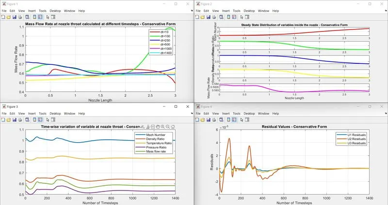
GRAPHS:
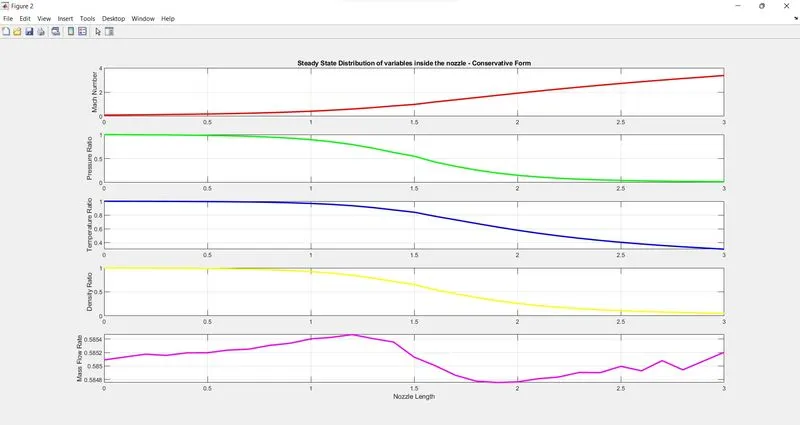
1) Steady State distribution of the primitive variables inside the nozzle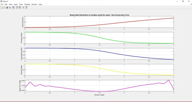

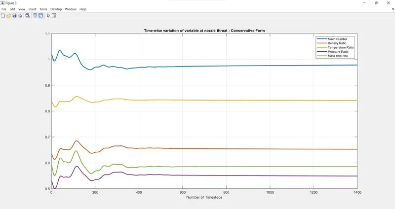
2) Time-wise variation of variable at nozzle throat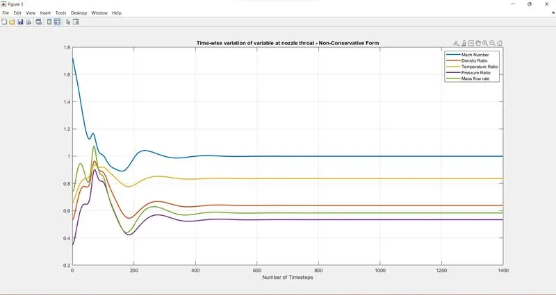

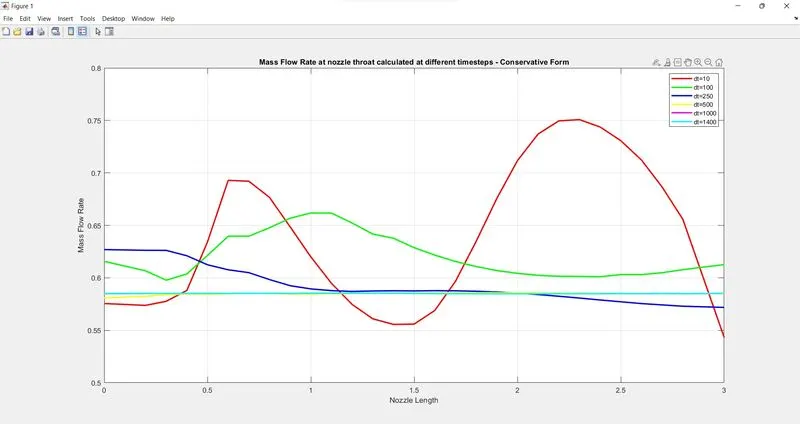
3) Mass Flow Rate at nozzle throat calculated at different timesteps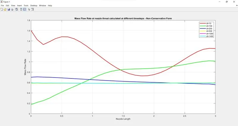


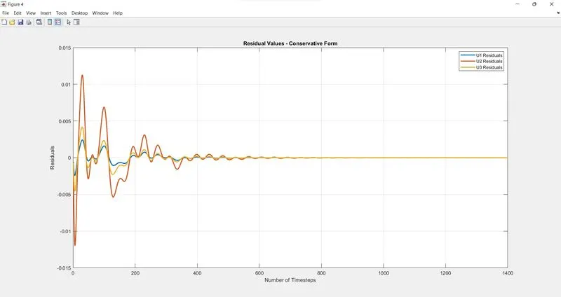
Residuals observed in the MacCormack Method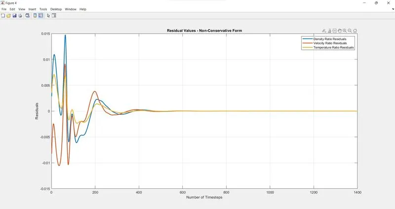


Grid Independence Test
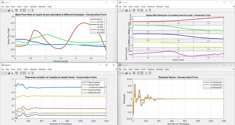
number of nodes = 31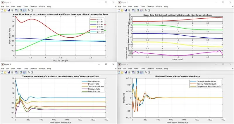


number of nodes = 61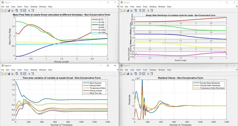


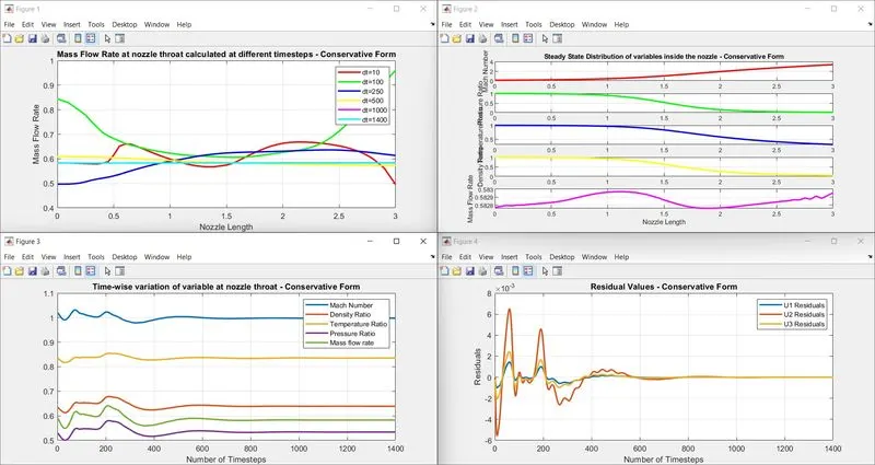
number of nodes = 91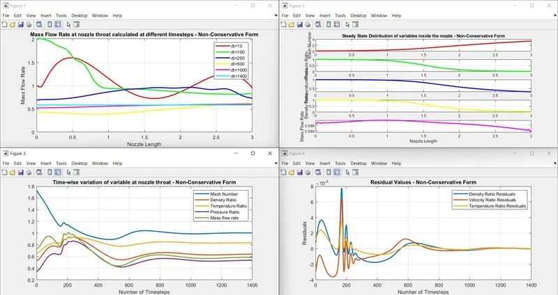

INFERENCES:
The isentropic flow simulation through a quasi 1D subsonic-supersonic nozzle has been executed as required. The required graphs are also plotted to show - the Steady State variation of the variables across the nozzle length, the time wise variation of these variables calculated at the nozzle throat against the number of iterations run in the simulation, the time wise variations of the mass flow rate calculated at the nozzle throat against the number iterations run in the simulation and the residual values observed throughout the simulation for both Non-Conservative and Conservative Forms respectively.
When the two forms of governing equations used here (Non-Conservative and Conservative) are compared we can conclude that they both result in a converging solution. However, while observing the Steady State Distribution of mass flow rate in the nozzle, the time wise variation of the variables within the nozzle throat and residual values, we can observe that in the Conservative form the variations in the initial few iterations result in a much smaller error than when compared to the ones observed in Non-Conservative form and hence also have smaller variations in the residual values with respect to the inital iterations. In CFD simulations the form of governing equations used has important implications on the solutions. if there are shocks, chemical reactions or any other sharp interfaces, then the Conservative form is used. However, there are various conditions, in many engineering situations Non-Conservative form is actually preferred while solving problems with shocks. For example, the Murman-Cole scheme, which uses a Non-Conservative form of governing equations, is highly preferred for transonic potential equations. It consists of a switch between central and upwind scheme.
Also a Grid Independence test has been performed on the simulations executed here. Three grids are considered having number of nodes = 31, 61 and 91. By comparing the graphical results in each of these cases, we can conclude that smaller the gridsize (i.e. greater the number of nodes) much lesser are the variations in the variables considered in the initial iterations i.e., the time wise variations are smaller when the gridsize is smaller. Also the residuals obtained in each form show smaller variations when smaller gridsizes are used. Hence, we can also say that the solution would converge faster if smaller gridsizes are used, however also to be noted is that the fact that this would slightly increase the computational requirement.