Week 3.5 - Deriving 4th order approximation of a 2nd order derivative using Taylor Table method

AIM: To derive the fourth order approximations for the second order derivative for the given function f(x)=exp(x)*cos(x) using Taylor Table method for the following schemes :
1) Central Difference
2) Skewed Right Sided Difference
3) Skewed Left Sided Difference
To write a program in MatLab to evaluate second order derivative of the given analytical function and compare it with the 3 numerical approximations derived. Also, plot the absolute error in each scheme against the range over which dx is considered.

DERIVATIONS:
In these derivations, the number nodes considered in the stencil are as per the rule:
N = P + Q - 1 for Central Difference Scheme and
N = P + Q for Skewed Difference Scheme
1) Central Difference Scheme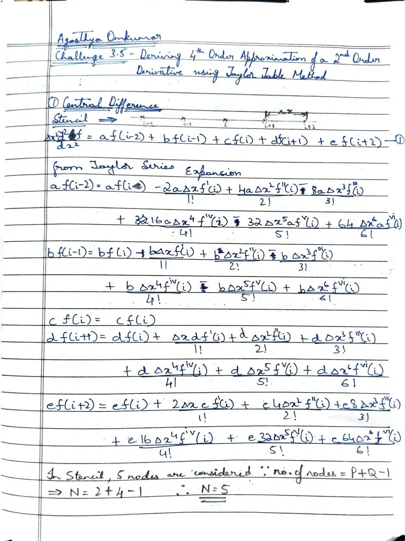



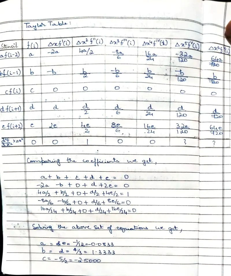
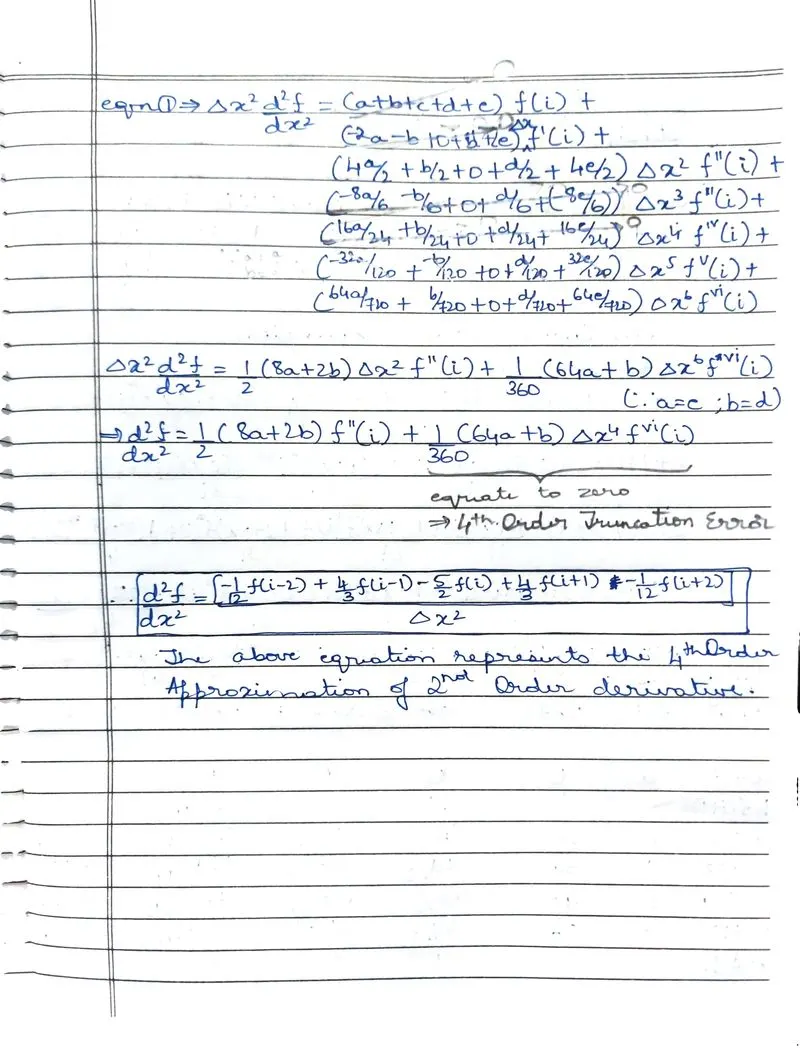
Here, the required functions are evaluated using Taylor Series formula and the terms are listed in Taylor Table as required to find the co-efficients. On solving the set of equations obtained from the Taylor Table (the equations are solved using Matrix method in MatLab), we determine the values of these co-efficients. On substituting them in the original equation, we get the fourth order approximation of the second order derivative in Central Difference Scheme.

2) Skewed Right Sided Difference Scheme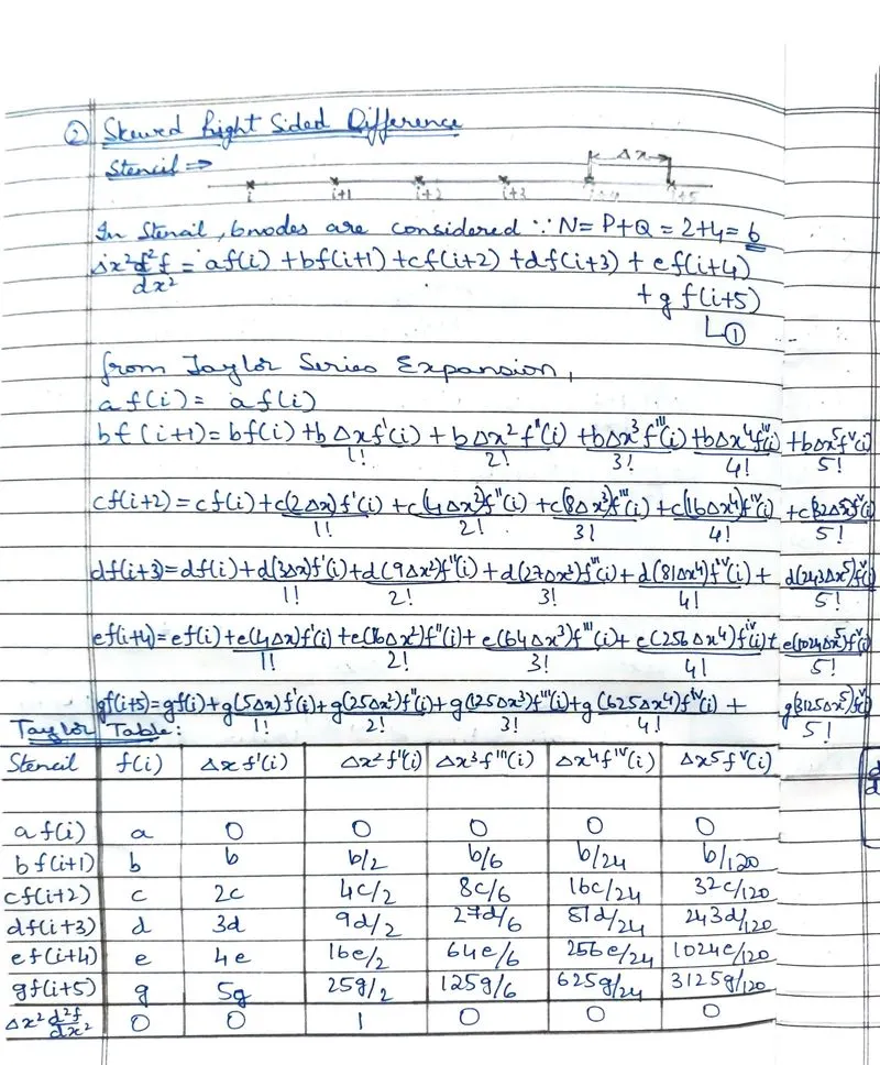


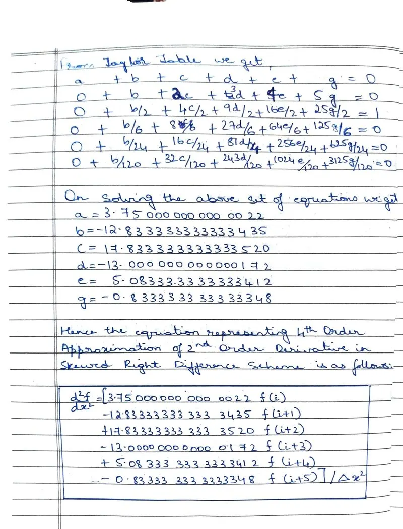
Here, the nodes taken in the stencil are not centralised and are taken to the right of the initial node 'i' successively. The required functions are then evaluated using Taylor Series formula and the terms are listed in Taylor Table as required to find the co-efficients. On solving the set of equations obtained from the Taylor Table (the equations are solved using Matrix method in MatLab), we determine the values of these co-efficients. The values for the co-efficients are taken as obtained in Matlab considering more digits to right of the decimal point than usual for accuracy because neglecting digits or rounding off results in inaccuracies we wish to avoid. On substituting them in the original equation, we get the fourth order approximation of the second order derivative in Skewed Right Sided Difference Scheme.

3) Skewed Left Sided Difference Scheme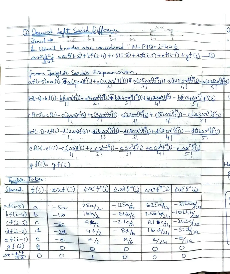


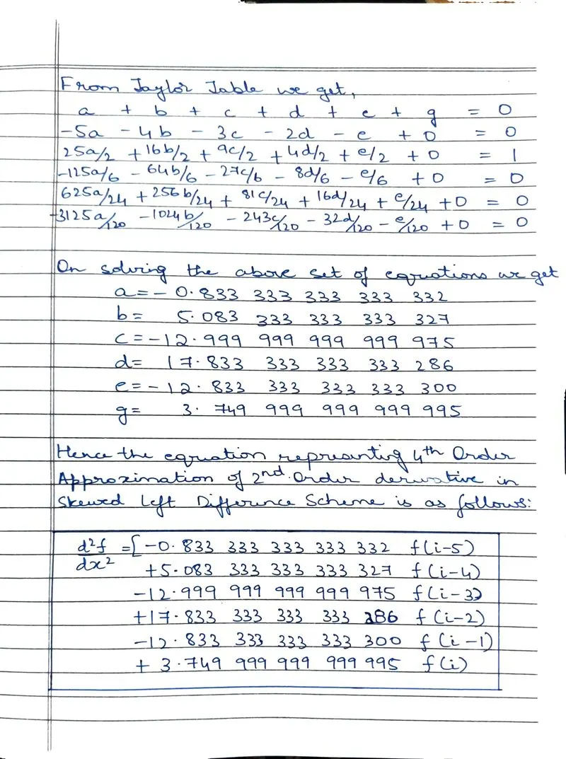
Here, the nodes taken in the stencil are not centralised and are taken to the left of the initial node 'i' successively. The required functions are then evaluated using Taylor Series formula and the terms are listed in Taylor Table as required to find the co-efficients. On solving the set of equations obtained from the Taylor Table (the equations are solved using Matrix method in MatLab), we determine the values of these co-efficients. The values for the co-efficients are taken as obtained in Matlab considering more digits to right of the decimal point than usual for accuracy because neglecting digits or rounding off results in inaccuracies we wish to avoid. On substituting them in the original equation, we get the fourth order approximation of the second order derivative in Skewed Left Sided Difference Scheme.

CODE:
Here, the code consists of 4 parts i.e., the main program and the three functions where error is calculated as per each of the formulae derived above. After the functions are properly defined, a for loop is created in the main program to calculate the error as per each scheme across the range over which dx is defined for the given function f(x)=exp(x)*cos(x). Then a log graph is plotted to compare the absolute error values in each of the three schemes with the appropriate legends and labels.
Function for Central Differencing Scheme

%function for error in Central Difference Approximation method
function error_CDA = CDA(x, dx)
%analytical function f(x) = exp(x)*cos(x)
%analytical derivative f''(x) = -2*exp(x)*sin(x)
a_derivative = -2*exp(x)*sin(x);
%co-efficient values from Taylor Table for Central Difference Approximation 
a = -1/12;
b = 4/3;
c = -5/2;
d = 4/3;
e = -1/12;
%numerical derivative CDA formula = ((a*f(x-2*dx)) + (b*f(x-dx)) + (c*f(x)) + (d*f(x+dx)) + (e*f(x+2*dx)))/dx^2
CDA = ((a*exp(x-2*dx)*cos(x-2*dx)) + (b*exp(x-dx)*cos(x-dx)) + (c*exp(x)*cos(x)) + (d*exp(x+dx)*cos(x+dx)) + (e*exp(x+2*dx)*cos(x+2*dx)))/dx^2;
error_CDA = abs(CDA - a_derivative);
end

Function for Skewed Right Sided Difference Scheme

%function for error in Skewed Right Side difference
function error_SRS = SRS(x, dx)
%analytical function f(x) = exp(x)*cos(x)
%analytical derivative f''(x) = -2*exp(x)*sin(x)
a_derivative = -2*exp(x)*sin(x);
%co-efficient values from Taylor Table for Skewed Right Side method
a = 3.750000000000022;
b = -12.833333333333435;
c = 17.833333333333520;
d = -13.000000000000172;
e = 5.083333333333412;
g = -0.833333333333348;
%numerical derivative SRS formula = ((a*f(x)) + (b*f(x+dx)) + (c*f(x+2*dx)) + (d*f(x+3*dx)) + (e*f(x+4*dx)) + (g*f(x+5*dx)))/dx^2
SRS = ((a*exp(x)*cos(x)) + (b*exp(x+dx)*cos(x+dx)) + (c*exp(x+2*dx)*cos(x+2*dx)) + (d*exp(x+3*dx)*cos(x+3*dx)) + (e*exp(x+4*dx)*cos(x+4*dx)) + (g*exp(x+5*dx)*cos(x+5*dx)))/dx^2;
error_SRS = abs(SRS - a_derivative);
end

Function for Skewed Left Sided Difference Scheme

function error_SLS = SLS(x, dx)
%function for error in Skewed Left Side difference
%analytical function f(x) = exp(x)*cos(x)
%analytical derivative f''(x) = -2*exp(x)*sin(x)
a_derivative = -2*exp(x)*sin(x);
%co-efficient values from Taylor Table for Skewed Left Side method
a = -0.833333333333332;
b = 5.083333333333327;
c = -12.999999999999975;
d = 17.833333333333286;
e = -12.833333333333300;
g = 3.749999999999995;
%numerical derivative SLS formula = ((a*f(x-5*dx)) + (b*f(x-4*dx)) + (c*f(x-3*dx)) + (d*f(x-2*dx)) + (e*f(x-1*dx)) + (g*f(x)))/dx^2
SLS = ((a*exp(x-5*dx)*cos(x-5*dx)) + (b*exp(x-4*dx)*cos(x-4*dx)) + (c*exp(x-3*dx)*cos(x-3*dx)) + (d*exp(x-2*dx)*cos(x-2*dx)) + (e*exp(x-dx)*cos(x-dx)) + (g*exp(x)*cos(x)))/dx^2;
error_SLS = abs(SLS - a_derivative);
end

Main Program

%Calculating fourth order approximation of second order derivative using Taylor Table
clear all
close all
clc
x = pi/3;
dx = linspace(pi/4000, pi/4, 40);
%for loop to calculate error throughout the range of dx in CD, SRS, SLS Methods
for i=1:length(dx)
    error_CDA(i) = CDA(x, dx(i));
    error_SRS(i) = SRS(x, dx(i));
    error_SLS(i) = SLS(x, dx(i));
end
%plotting graph to comapre the error values in each method
figure(1)
loglog(dx, error_CDA, LineWidth=2)
hold on 
loglog(dx, error_SRS, 'r', LineWidth=2)
hold on
loglog(dx, error_SLS, 'g', LineWidth=2)
xlabel('dx')
ylabel('Absolute Error')
legend('Central Difference of 4th Order', 'Skewed Right Sided Difference of 4th Order', 'Skewed Left Sided Difference of 4th Order')

GRAPH: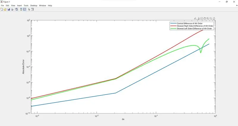

INFERENCES:
One of the things that can be clearly observed is that all three lines have similar slopes and it can also be observed that beyond a certain value (less than 10^(-2)) the slope of each of the curves changes and the error value is greater than expected. This is because sometimes the error produced by higher order schemes is greater than those produced by lower order schemes because of the round-off error being higher. Hence a higher order scheme may not always be desirable.

The error in Central Difference Scheme is noticeably lesser than the error values obtained in the skewed schemes, hence it would be highly preferable to use Central Difference Scheme rather than a skewed scheme. Also in Central Difference Scheme, the convergence rate is faster than in other Finite Difference Methods.

However, when seen from a physics point of view, Skewed Schemes have an advantage over the Central Difference Schemes. This advantage comes with respect to choosing the nodes of the stencil, there may be instances where we may not be able to consider points behind or ahead of the initial point of consideration 'i'. In such cases, Central Difference Scheme cannot be used and hence a Skewed Scheme will have to be used. An example could be in fluid mechanics, when flow has to be considered from a certain point behind which there exists no flow; in such a case Skewed Right Sided Difference Scheme is very useful because there is no information about the nodes prior to source of flow. Another example could be where air flow is considered against the frontal surface area of an automobile where information regarding the flow is available only behind the point of consideration (solid surface of the vehicle); in such case Skewed Left Sided Difference Scheme is very useful because information regarding the flow is not available beyond the physical boundary.