Week 9 - FVM Literature Review

The finite difference method is based upon the differential form of the PDE that govern fluid flow and heat transfer. However, the finite volume method is a numerical method applied to transport equations governing fluid flow and heat transfer in the integral form. The control volume integration expresses the conservation of relevant properties for each finite size cell. That is the main reason that it is widely used in many softwares.

Other differences about FVM (finite volume method) and FDM (finite difference method) is that the FDM store the value of the dependant value in points, instead of FVM that the dependant values are in the center of a volume. Pherhaps the use of FVM does not require structured mesh, which could make complex if the unstructured mesh are present in the FDM.

As we know, OpenFOAM has a large amount of codes, that contains discretization techniques that is suitable to the different transport terms: convection, diffussion and so on. Inside the library, we stand out the use of interpolation schemes and flux limiters.

We can do the example of 1D linear heat conduction equation.

We extract one problem from (Versteeg Malalasekera 2ed, 2007), it consists of a large plate of thickness L=2cm with constant thermal conductivity `alpha=0.5W/(m.K)`and unifirm heat generation `q=1000 (kW)/(m^3)`. The faces A and B are at temperatures of 100 and 200°C respectively.

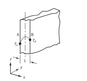
The governing equation is:

`(d)/(dx)(alpha(dT)/(dx))+q=0`

The integration of the governing equation over a control volume (it is represented in the figure above, the shaded region) gives

`int_(triangleV)(d)/(dx)(alpha(dT)/(dx))dV+int_(triangleV)qdV=0`

`[(alphaA(dT)/(dx))_e-(alphaA(dT)/(dx))_w]+qtriangleV=0`

`[alpha_eA((dT)/(dx))_e-alpha_wA((dT)/(dx))_w]+qtriangleV=0`

The gradients `(dT)/(dx)`over the faces of the control volume are discretized through the gradient scheme, which numerically represent the gradient in a face.

`((dT)/(dx))_e=((T_E-T_P)/(deltax))`

`((dT)/(dx))_w=((T_P-T_W)/(deltax))`

Interpolation schemes transform cell-centre quantities to face centres. It is applied to the thermal conductivity.

`alpha_e=0.5*(alpha_E+alpha_P)`

`alpha_w=0.5*(alpha_W+alpha_P)`

However, in this case, the thermal conductivity is constant, so it doesn't apply.

The discretized equation gives:

`[alphaA((T_E-T_P)/(deltax))-alphaA((T_P-T_W)/(deltax))]+qAdeltax=0`

With some rearrangements and the applications of iterative methods it is possible to solve the problem. We use the Gauss Seidel method to solve the system iteratively. It is solved in MatLAB code.

clear all
close all
clc

%Define inputs
L=0.02;
k=0.5;
A=1;
q=1000000;
tol=1e-4; %min tolerance for iterative solvers 

%Creating mesh
n=5;
dx=L/(n);
x=linspace(0,L-dx,n)+dx/2;
x=[0 x L];

%Initial temperature
Ta=100;
Tb=200;
T=zeros(1,n+2);
T(1)=Ta;
T(end)=Tb;

error=9e9;
Told=T;

%Gauss Seidel method
    n_iter=1;
%Convergence loop
while(error>tol)
    for i=2:n+1
        if i==2
            aw=0;
            ae=k*A/dx;
            Sp=-2*k*A/dx;
            Su=q*A*dx+2*k*A/dx*Ta;
            ap=aw+ae-Sp;
        elseif i>=3 && i<=n
            aw=k*A/dx;
            ae=k*A/dx;
            Sp=0;
            Su=q*A*dx;
            ap=aw+ae-Sp;
        else
            aw=k*A/dx;
            ae=0;
            Sp=-2*k*A/dx;
            Su=q*A*dx+2*k*A/dx*Tb;
            ap=aw+ae-Sp;
        end     
        T(i)=aw/ap*T(i-1)+ae/ap*Told(i+1)+Su/ap;   
    end  
    error=max(abs(Told-T));
    Told=T;
    n_iter=n_iter+1;
end

%Analitycal solution
T_exact=((Tb-Ta)/L+q/(2*k)*(L-x)).*x+Ta;

fprintf('%6s %12s %10s %10s\n','x','exact','fvm','error');
for j=2:n+1
    fprintf('%6.4f %12.4f %10.4f %10.4f\n',x(j),T_exact(j),T(j),abs(T(j)-T_exact(j))/T_exact(j)*100);
end

plot(x,T_exact)
hold on
scatter(x,T)
grid on
legend('Exact','Numerical')
xlabel('Distance (m)')
ylabel('Temperature (°C)')

The results are below:

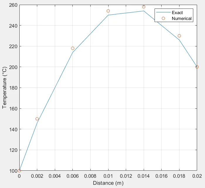
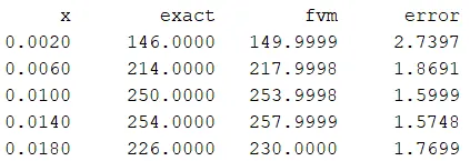
In this case, the flux of T leaving the control volume across a certain face `(alphaA(dT)/(dx))_e` is equal to the flux of T entering the adjacent control volume `(alphaA(dT)/(dx))_w` trhough the same face. This means that the discretizations schemes used satisfiy the property of conservativeness.

There are cases where the gradients have huge values, for example this case (figure from Versteeg Malalasekera 2ed, 2007):

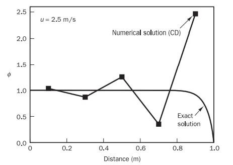
Theoretically, numerical results may be obtained more accurate when the number of computational cells are large, but in practical calculations we can only use a finite number of cells. In the figure above we can see wiggles, this is a case when discretization schemes does not accomplish the property of boundedness. In order to do that, there are some functions that multiply elements of the difference equations (algebraic form of partial derivatives), those elements are related with the flux terms. These functions limit gradients by modifying the flux terms in the difference equations, they are called flux limiters.