Week 11 - Simulation of Flow through a pipe in OpenFoam
Pre-analysis
In this project, namely a simulation of flow though a pipe in OpenFOAM, an axi-symmetric flow is simulated applying the wedge boundary conditions. The flow is laminar and the Reynolds number is 2100. The numerical results are then compared with the Hagen Poiseuille fully developed flow.
Because this case is about an internal flow, it means inside walls, the viscous effect is present. As the inviscid flow enters to the pipe, the axial velocity near the walls tend to retard and the velocity at the center is increased since the continuity principle (incompressible flow). This can be shown in the figure below (Source: Fluid Mechanics. Frank M. White. Seventh Edition).
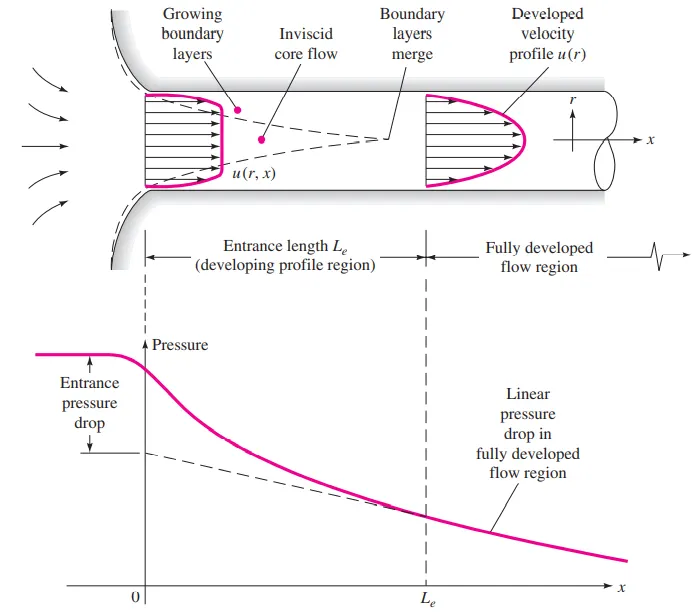
When the boundary layers merge, the flow becomes entirely viscous. An entrance length is defined as the developing profile region, so downstream this length, a fully developed region is created, where the velocity profile and shear stress is constant, and the pressure drops linearly with x. The entrance length is defined as:
`(Le)/(D)=0.06*Re`
The fully developed region makes the velocity profile constant in a parabolic form, that is called the Hagen Poiseuille flow, which equations is defined in cylindrical coordinates.
Continuity equation `(del)/(delz)(v_z)=0`
r-momentum equation `(del p)/(del r)=0`
z-momentum equation `(mu)/(r)(d)/(dr)(r(dv_z)/(dr))=(dp)/(dz)`
The Hagen Poiseuille equation of the velocity profile is:
`v_z=(-(dp)/(dz))(1)/(4mu)(R^2-r^2)`
In our case, the average velocity is assumed in order to satisfy the Reynolds number of 2100. The equation above is rearranged:
`(v_z)/(V_(avg))=2(R^2-r^2)`, also `V_(max)=2V_(avg)`
Geometry
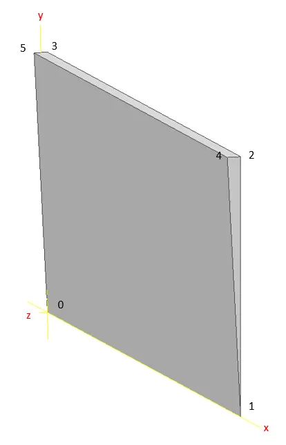
The following parameters are assumed at first, the angle equal to 3º and the diameter 0.5m, because the Reynolds number has to be 2100, the entrance length is calculated in order to estimate the lentgh of the pipe.
`(Le)/(0.5)=0.06*2100`
So Le=63m, the total length of the pipe is defined as 80m, to show the fully developed region. The geometry is like the figure below.
Mesh
The grid is executed with blockMesh of OpenFOAM, and the blockMeshDict file is created by a code in MatLAB. We come up with the boundary names as the figure below.
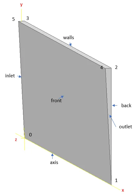
We stand out that in the code there are some parameters that take part of the simulation, that is not relevant with the creation of the blockMeshDict file.
clear all
close all
clc

%Input_values
alpha=3;
D=0.5;
L=80;
z=D/2*sin(alpha/2*pi/180);
y=D/2*cos(alpha/2*pi/180);

%Reynolds number
Re=2100;
v=2.1;
nu=v*D/Re;

%Entrance length
Le=0.06*Re*D;

%Courant number
dt=0.05;
nx=400;
ny=10;
dx=L/nx;
dy=y/ny;
Cou=0.5*v*dt/dx;

Vmax=2*v;
R=D/2;
r=linspace(0,R,20);
v_prof=Vmax*(1-r.^2/R^2);

%blockMeshDict file
file=fopen('blockMeshDict.txt','w');
fprintf(file,'%s\n','FoamFile');
fprintf(file,'%s\n','{');
fprintf(file,'%s\n','    format      ascii;');
fprintf(file,'%s\n','    class       dictionary;');
fprintf(file,'%s\n','    object      blockMeshDict;');
fprintf(file,'%s\n','}');
fprintf(file,'%s\n','convertToMeters 1;');
fprintf(file,'%s\n','vertices');
fprintf(file,'%s\n','(');
fprintf(file,'%s%d %d %d%s\n','    (',0,0,0,')');
fprintf(file,'%s%d %d %d%s\n','    (',L,0,0,')');
fprintf(file,'%s%d %.4f %.4f%s\n','    (',L,y,-z,')');
fprintf(file,'%s%d %.4f %.4f%s\n','    (',0,y,-z,')');
fprintf(file,'%s%d %.4f %.4f%s\n','    (',L,y,z,')');
fprintf(file,'%s%d %.4f %.4f%s\n','    (',0,y,z,')');
fprintf(file,'%s\n',');');
fprintf(file,'%s\n','blocks');
fprintf(file,'%s\n','(');
fprintf(file,'%s%d %d %d %d %d %d %d %d%s%d %d %d%s%d %d %d%s\n','    hex (',0,3,5,0,1,2,4,1,') (',ny,1,nx,') simpleGrading (',1,1,1,')');
fprintf(file,'%s\n',');');
fprintf(file,'%s\n','boundary');
fprintf(file,'%s\n','(');
fprintf(file,'%s\n','    inlet');
fprintf(file,'%s\n','    {');
fprintf(file,'%s\n','        type wall;');
fprintf(file,'%s\n','        faces');
fprintf(file,'%s\n','        (');
fprintf(file,'%s%d %d %d %d%s\n','            (',0,5,3,0,')');
fprintf(file,'%s\n','        );');
fprintf(file,'%s\n','    }');
fprintf(file,'%s\n','    outlet');
fprintf(file,'%s\n','    {');
fprintf(file,'%s\n','        type wall;');
fprintf(file,'%s\n','        faces');
fprintf(file,'%s\n','        (');
fprintf(file,'%s%d %d %d %d%s\n','            (',1,2,4,1,')');
fprintf(file,'%s\n','        );');
fprintf(file,'%s\n','    }');
fprintf(file,'%s\n','    walls');
fprintf(file,'%s\n','    {');
fprintf(file,'%s\n','        type wall;');
fprintf(file,'%s\n','        faces');
fprintf(file,'%s\n','        (');
fprintf(file,'%s%d %d %d %d%s\n','            (',2,3,5,4,')');
fprintf(file,'%s\n','        );');
fprintf(file,'%s\n','    }');
fprintf(file,'%s\n','    front');
fprintf(file,'%s\n','    {');
fprintf(file,'%s\n','        type wedge;');
fprintf(file,'%s\n','        faces');
fprintf(file,'%s\n','        (');
fprintf(file,'%s%d %d %d %d%s\n','            (',0,1,4,5,')');
fprintf(file,'%s\n','        );');
fprintf(file,'%s\n','    }');
fprintf(file,'%s\n','    back');
fprintf(file,'%s\n','    {');
fprintf(file,'%s\n','        type wedge;');
fprintf(file,'%s\n','        faces');
fprintf(file,'%s\n','        (');
fprintf(file,'%s%d %d %d %d%s\n','            (',0,3,2,1,')');
fprintf(file,'%s\n','        );');
fprintf(file,'%s\n','    }');
fprintf(file,'%s\n','    axis');
fprintf(file,'%s\n','    {');
fprintf(file,'%s\n','        type empty;');
fprintf(file,'%s\n','        faces');
fprintf(file,'%s\n','        (');
fprintf(file,'%s%d %d %d %d%s\n','            (',0,1,1,0,')');
fprintf(file,'%s\n','        );');
fprintf(file,'%s\n','    }');
fprintf(file,'%s\n',');');
fclose(file);
The output is below, note the type of boundary wedge in the front and back face:
FoamFile
{
    format      ascii;
    class       dictionary;
    object      blockMeshDict;
}
convertToMeters 1;
vertices
(
    (0 0 0)
    (80 0 0)
    (80 0.2499 -0.0065)
    (0 0.2499 -0.0065)
    (80 0.2499 0.0065)
    (0 0.2499 0.0065)
);
blocks
(
    hex (0 3 5 0 1 2 4 1) (10 1 400) simpleGrading (1 1 1)
);
boundary
(
    inlet
    {
        type wall;
        faces
        (
            (0 5 3 0)
        );
    }
    outlet
    {
        type wall;
        faces
        (
            (1 2 4 1)
        );
    }
    walls
    {
        type wall;
        faces
        (
            (2 3 5 4)
        );
    }
    front
    {
        type wedge;
        faces
        (
            (0 1 4 5)
        );
    }
    back
    {
        type wedge;
        faces
        (
            (0 3 2 1)
        );
    }
    axis
    {
        type empty;
        faces
        (
            (0 1 1 0)
        );
    }
);
If we execute the command blockMesh in OpenFOAM we obtain the following:
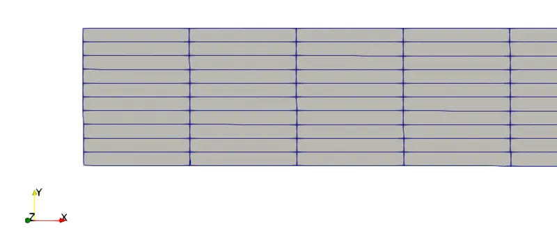
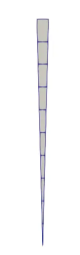
The number of cells along x axis is 10 and along y axis is 400. There are in total 4420 cells. The simpleGrading is (1 1 1)
Model setup
We choose a transient simulation. Because the flow is laminar and incompressible, the icoFoam solver is chosen.
Boundary conditions
- Inlet: uniform velocity v=2.1, which is the average velocity. That is because the velocity at the entrance belongs to an inviscid flow.
- Outlet: uniform pressure p=0, note that in OpenFOAM the pressure is defined as the dymanic pressure.
- The walls are defined as no slip conditions.
U file
/*--------------------------------*- C++ -*----------------------------------*\
  =========                 |
  \\      /  F ield         | OpenFOAM: The Open Source CFD Toolbox
   \\    /   O peration     | Website:  https://openfoam.org
    \\  /    A nd           | Version:  9
     \\/     M anipulation  |
\*---------------------------------------------------------------------------*/
FoamFile
{
    format      ascii;
    class       volVectorField;
    object      U;
}
// * * * * * * * * * * * * * * * * * * * * * * * * * * * * * * * * * * * * * //

dimensions      [0 1 -1 0 0 0 0];

internalField   uniform (0 0 0);

boundaryField
{
    inlet
    {
        type            fixedValue;
        value           uniform (2.1 0 0);
    }

    outlet
    {
        type            zeroGradient;
    }

    walls
    {
        type            noSlip;
    }

    front
    {
        type            wedge;
    }

    back
    {
        type            wedge;
    }
}

// ************************************************************************* //
p file
/*--------------------------------*- C++ -*----------------------------------*\
  =========                 |
  \\      /  F ield         | OpenFOAM: The Open Source CFD Toolbox
   \\    /   O peration     | Website:  https://openfoam.org
    \\  /    A nd           | Version:  9
     \\/     M anipulation  |
\*---------------------------------------------------------------------------*/
FoamFile
{
    format      ascii;
    class       volScalarField;
    object      p;
}
// * * * * * * * * * * * * * * * * * * * * * * * * * * * * * * * * * * * * * //

dimensions      [0 2 -2 0 0 0 0];

internalField   uniform 0;

boundaryField
{
    inlet
    {
        type            zeroGradient;
    }

    outlet
    {
        type            fixedValue;
        value           uniform 0;
    }

    walls
    {
        type            zeroGradient;
    }

    front
    {
        type            wedge;
    }

    back
    {
        type            wedge;
    }
}

// ************************************************************************* //
Transport properties
Because the Reynolds number is 2100 and the velocity is 2.1, the dymanic viscosity is `nu=5*10^(-4)m^2/s`.
Time of simulations, solvers and Courant number
Because we use the cavity tutorial, the fvschemes and fvsolution files are in default. Only in controlDict file we change the values to dt=0.05, and the endTime to 40.
To estimate the courant number at the iteration 0, the formula is reduced to:
`Co=0.5*v(dt)/(dx)`
The v=2.1 m/s, dt=0.05 and dx=0.2, so the value of Co=0.2625, which is less than 1.
After the execution of icoFoam solver in the terminal, with the endTime of 40 we can obtain the following residuals.
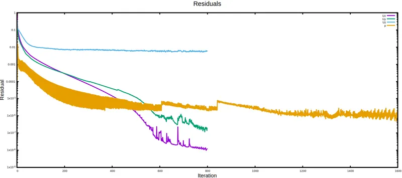
We can see that the residuals for Ux and Uy are less than 10^-6. The max. Courant number is 1.03457.
Numerical results
The velocity contour at the outlet region is like the figure below, we can see that we have a maximum velocity at the center with a value almost twice the average velocity.
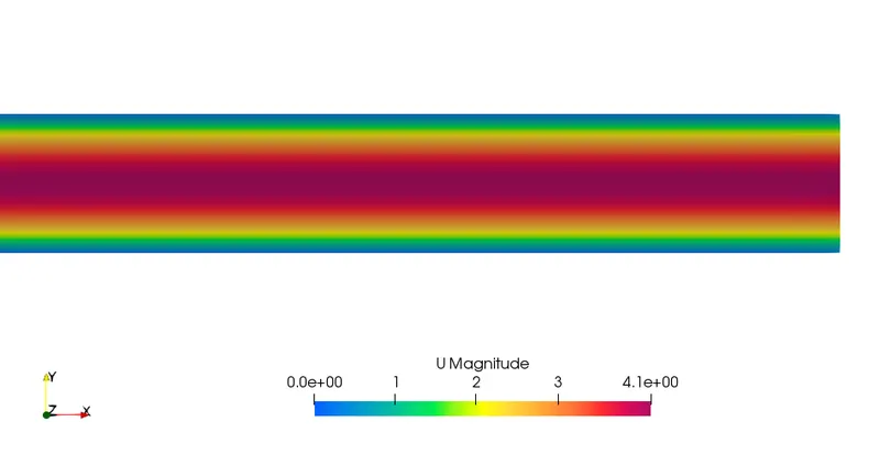
The velocity profiles at different values of x axis are shown below, we can see the development of the parabolic form when the value x increase
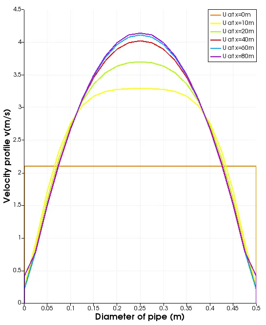
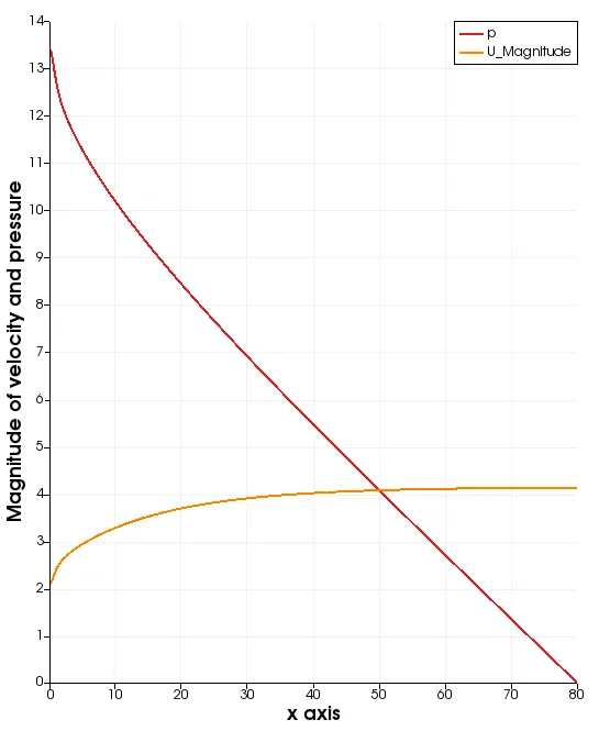
In the figure below we can see that the pressure changes until reach a linear pressure drop. Also the velocity at the center tends to be constant and twice the average velocity.
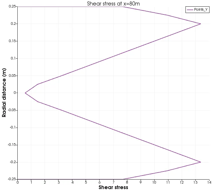
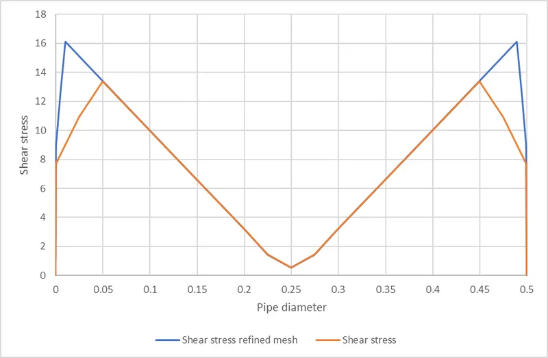
The shear stress profile is obtained and shown in the figure below, we assume a value of density equal to 1000.
Validation
First, we compare the velocity profile at x=80m numerically with the exact solution of the profile that provides from the Hagen Poiseuille equation for velocity.
`(v_z)/(V_(avg))=2(R^2-r^2)`
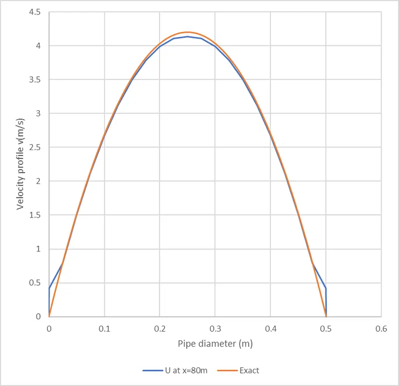
We can see that the numerical result is pretty close to the exact solution, the error is most likely due to the truncation error that provides from dx or dy, so the mesh refinement is formulated, also we will refine the mesh at the walls.
Mesh refinement
We refine the mesh modifying the following
blocks
(
    hex (0 3 5 0 1 2 4 1) (20 1 400) simpleGrading (0.2 1 1)
);
Prior to that, we define nx=800 cells, and the Courant number in the iteration zero is estimated to 0.525, but the max. Courant number in the following iterations tends to increase rapidly, triggering instabilities. With a value of nx=600 the max. Courant number is approximately 1.6, in the residuals plot we observe some fluctuations, so finally we don't modify the nx. We can state nx=800 cells, but the dt has to decrease.
Velocity profile
We can see that the velocity profile is nearer to the exact solution instead to the first mesh posed. Also the refinement allows that the profile is almost close to the exact solution. We can obtain the maximum value of velocity closer to the exact solution, if we refine the mesh, but it brings to reduce dt, in order to stabilize the solution.
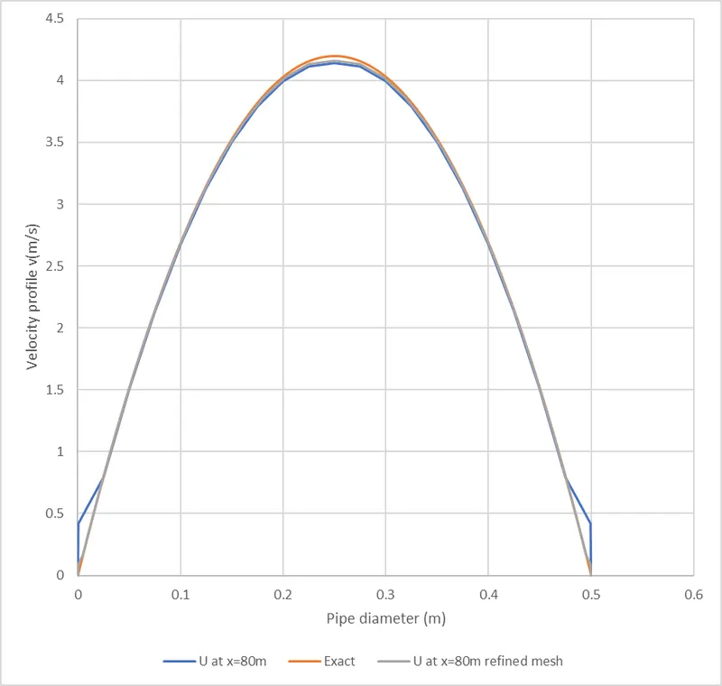
The maximum value of velocity with the first mesh is 4.138 and with the refined mesh is 4.161 m/s.
Shear stress
The shear stress is graphed below, both numerical results, the first and refined mesh.
The shear stress at the wall (exact) is
`tau_(wall)=(4muV_(avg))/(R)`
If we replace the values, we obtain a magnitude of 16.8, the maximum numerical values obtained are 13.374 for the first mesh and 16.1058 for the refined mesh, if we refine the mesh even more at the walls, we can obtain a pretty close value.
Entrance length
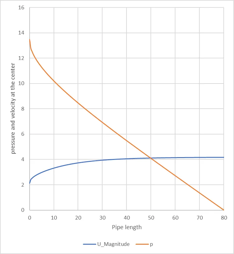
We can see from the figure that the maximum velocity is almost constant at the length of 63m, which is the value obtained in the pre-analysis, indeed the pressure drop is linear in this region, as we can see in the figure.