Week 7 - Simulation of a 1D Super-sonic nozzle flow simulation using Macormack Method

The present challenge deals with the quasi-one-dimensional flow through a convergent-divergent nozzle, which is applied in rocket engines.

A steady, isentropic flow through the nozzle is considered. The flow at the inlet comes from a reservoir where the pressure and temperature are the stagnation values, the cross sectional area of the reservoir is large, thus the velocity is very small. The flow expand isentropically to supersonic speeds a the nozzle exit.

The flow properties are uniform across the section of the nozzle, so we make an assumption that these properties vary only with x. Such flow is defined as quasi-one dimensional flow.

Equations for quasi-one dimensional, steady, isentropic flow are solved analytically. The mach number variation is a result of this. It is expressed by the following:

`(A/A^*)^2=1/M^2[2/(gamma-1)(1+(gamma-1)/2(M^2))]^((gamma+1)/(gamma-1))`

Through this expression, is possible to obtain other to obtain the variation of pressure, density and temperature as a function of Mach number (hence as a function of A/A*, thus x).

CFD solution of subsonic-supersonic isentropic nozzle flow: MacCormack technique

We will set up a time-marching, finite-difference solution for the quasi-one-dimensional nozzle flow

Governing flow equations are implemented in terms of partial differential equations.

• Continuity equation suitable for unsteady, quasi one-dimensional flow.

`(del(rhoA))/(delt)+(del(rhoAV))/(delx)=0`

• Conservation form of the momentum equation for quasi one-dimensional flow.

`(del(rhoVA))/(delt)+(del(rhoV^2A))/(delx)=-A(delp)/(delx)`

• Non Conservation form of the momentum equation for quasi one-dimensional flow.

`rho(delV)/(delt)+rhoV(delV)/(delx)=-(delp)/(delx)`

• Conservation form of the internal energy equation for quasi one-dimensional flow.

`(del(rhoeA))/(delt)+(del(rhoVeA))/(delx)=-p(delAV)/(delx)`

• Non Conservation form of the internal energy equation for quasi one-dimensional flow.

`rho(dele)/(delt)+rhoV(dele)/(delx)=-p(delV)/(delx)-pV(dellnA)/(delx)`

Then, we proceed to solve these problem with the nonconservative and conservative forms of these equations.

1. The setup of nonconservative form of quasi-one-dimensional flow through a convergent-divergent nozzle

Governing equations expressed in terms of nondimensional variables.

`(delrho)/(delt)=-rho(delV)/(delx)-rhoV(dellnA)/(delx)-V(delrho)/(delx)`

`(delV)/(delt)=-V(delV)/(delx)-1/gamma((delT)/(delx)+T/rho(delrho)/(delx))`

`(delT)/(delt)=-V(delT)/(delx)-(gamma-1)T((delV)/(delx)+V(dellnA)/(delx))`

The finite difference equations

Creating the mesh, we establish 31 points over the 1d domain in a large of L=3. Each grid has the same value.

Initial conditions

`rho=1-0.3146x`

`T=1-0.2314x`

`V=(0.1+1.09x)T^(0.5)`

Area: `1+2.2(x-1.5)^2`

MacCormack method

• Predictor step: `((delf)/(delt))_p` Use the forward difference of the space derivatives.
• Solution update: `f^u=f_(old)+((delf)/(delt))_p`
• Corrector step: `((delf)/(delt))_c` Use the backward difference of the space derivatives.
• Average of derivatives: `((delf)/(delt))_(avg)=0.5(((delf)/(delt))_c+((delf)/(delt))_p)`
• Next value: `f^(2nd)=f_(old)+((delf)/(delt))_(avg)`

Calculation of time step

Considering the stability constraints, where C is the courant number, the time step is expressed by:

`(trianglet)_i^t=C(trianglex)/(a_i^t+V_i^t)` at a given grid point at a given time step.

Calculate the `(trianglet)_i^t` at all the grid points, and the choose the minimun value for use.

`trianglet=min(trianglet_1^t,trianglet_2^t,...,trianglet_N^t)`

Boundary conditions

• Inflow:

`V_1=2V_2-V_3` floating value

`rho_1=1`fixed, independent of time

`T_1=1` fixed, independent of time

• Outflow

`V_N=2V_(N-1)-V_(N-2)` floating value

`rho_N=2rho_(N-1)-rho_(N-2)` floating value

`T_N=2T_(N-1)-T_(N-2)` floating value

The function to solve the subsonic-supersonic flow through the convergent-divergent nozzle numerically is implemented following the procedure above, in the nonconservative form.

function [x,rho,v,T,p,M,m,rho_throat,T_throat,p_throat,M_throat,m_time]=non_conservative_subsonic_supersonic_nozzle_function(L,n,nt,C)
%Creating mesh
dx=L/(n-1);
x=linspace(0,L,n);
%Initial profiles
rho=1-0.3146*x;
T=1-0.2314*x;
v=(0.1+1.09.*x).*T.^(1/2);
%Area
A=1+2.2*(x-1.5).^2;
%Mass flow distribution dt=0
rho_initial=rho;
v_initial=v;
m_time=ones(6,n);
m_time(1,:)=rho_initial.*v_initial.*A;
%Count
count=2;
%Fluid: air
gamma=1.4;
%MacCormack Method
%Time-marching approach
for k=1:nt
    %First values
    rho_old=rho;
    v_old=v;
    T_old=T;

    for i=2:n-1
        %space derivatives
        dvdx=(v(i+1)-v(i))/dx;
        drhodx=(rho(i+1)-rho(i))/dx;
        dTdx=(T(i+1)-T(i))/dx;
        dlogAdx=(log(A(i+1))-log(A(i)))/dx;        
        %Predictor step
        drhodt_p(i)=-rho(i)*dvdx-rho(i)*v(i)*dlogAdx-v(i)*drhodx;
        dvdt_p(i)=-v(i)*dvdx-1/gamma*(dTdx+T(i)/rho(i)*drhodx);
        dTdt_p(i)=-v(i)*dTdx-(gamma-1)*T(i)*(dvdx+v(i)*dlogAdx);
    end
    %dt calculation
    delt=C*dx./(v+(T).^0.5);
    dt=min(delt);
    for i=2:n-1
        %Solution update
        rho(i)=rho(i)+drhodt_p(i)*dt;
        v(i)=v(i)+dvdt_p(i)*dt;
        T(i)=T(i)+dTdt_p(i)*dt;
    end
    for i=2:n-1
        %space derivatives
        dvdx=(v(i)-v(i-1))/dx;
        drhodx=(rho(i)-rho(i-1))/dx;
        dTdx=(T(i)-T(i-1))/dx;
        dlogAdx=(log(A(i))-log(A(i-1)))/dx;
        %Corrector step
        drhodt_c(i)=-rho(i)*dvdx-rho(i)*v(i)*dlogAdx-v(i)*drhodx;
        dvdt_c(i)=-v(i)*dvdx-1/gamma*(dTdx+T(i)/rho(i)*drhodx);
        dTdt_c(i)=-v(i)*dTdx-(gamma-1)*T(i)*(dvdx+v(i)*dlogAdx);
        %Average of derivatives
        drhodt_avg(i)=0.5*(drhodt_p(i)+drhodt_c(i));
        dvdt_avg(i)=0.5*(dvdt_p(i)+dvdt_c(i));
        dTdt_avg(i)=0.5*(dTdt_p(i)+dTdt_c(i));
    end
    for i=2:n-1
        %Next value
        rho(i)=rho_old(i)+drhodt_avg(i)*dt;
        v(i)=v_old(i)+dvdt_avg(i)*dt;
        T(i)=T_old(i)+dTdt_avg(i)*dt;
    end
    %Applying boundary conditions
    %Inflow boundary condition
    v(1)=2*v(2)-v(3);
    %Outflow boundary conditions
    rho(n)=2*rho(n-1)-rho(n-2);
    v(n)=2*v(n-1)-v(n-2);
    T(n)=2*T(n-1)-T(n-2);
    
    %Pressure
    p=rho.*T;
    %Mach number
    M=v./(T).^0.5;
    %mass flow
    m=rho.*v.*A;
    
    %Primitive values at the throat
    rho_throat(k)=rho((n+1)/2);
    T_throat(k)=T((n+1)/2);
    p_throat(k)=p((n+1)/2);
    M_throat(k)=M((n+1)/2);
    
    %Return mass flow rates at different time steps
    if ismember(k,[50 100 150 200 700])==1
            m_time(count,:)=m;
            count=count+1;
    end
end
end

2. The setup of conservative form of quasi-one-dimensional flow through a convergent-divergent nozzle

Governing equations expressed in terms of nondimensional variables.

`(del(rhoA))/(delt)+(del(rhoVA))/(delx)=0`

`(del(rhoAV))/(delt)+(del(rhoV^2A+1/gammapA))/(delx)=1/gammap(delA)/(delx)`

`(del(rho(e/(gamma-1)+gamma/2V^2)A))/(delt)+(del(rho(e/(gamma-1)+gamma/2V^2)VA+pAV))/(delx)=0`

Rewrite the equations above

`(delU1)/(delt)=-(delF1)/(delx)`

`(delU2)/(delt)=-(delF2)/(delx)+J2`

`(delU3)/(delt)=-(delF3)/(delx)`

Primitive values

`rho=(U1)/(A)`

`V=(U2)/(U1)`

`T=(gamma-1)((U3)/(U1)-gamma/2V^2)`

`p=rhoT`

"Pure" form of the flux terms

`F1=U2`

`F2=(U2^2)/(U1)+(gamma-1)/gamma(U3-gamma/2(U2^2)/(U1))`

`F3=gamma(U2U3)/(U1)+gamma(gamma-1)/2(U2^3)/(U1^2)`

`J2=1/gammarhoT(delA)/(delx)`

`J2=(gamma-1)/gamma(U3-gamma/2(U2^2)/(U1))(dellnA)/(delx)`

The finite difference equations

Creating the mesh, we establish 31 points over the 1d domain in a large of L=3. Each grid has the same value.

Initial conditions

For `0<=x<=0.5`

`rho=1`

`T=1`

For `0.5<=x<=1.5`

`rho=1-0.366(x-0.5)`

`T=1-0.167(x-0.5)`

For `1.5<=x<=3.5`

`rho=0.634-0.3879(x-1.5)`

`T=0.833-0.3507(x-1.5)`

Area: `1+2.2(x-1.5)^2`

MacCormack method

The same as the nonconservative form

Calculation of time step

The same as the nonconservative form

Boundary conditions

• Inflow:

`U1_1=(rhoA)_1=A_1` fixed value

`U2_1=2U2_2-U2_3` floating value

`U3=U1(T/(gamma-1)+gamma/2V^2)`

• Outflow

`U1_N=2U1_(N-1)-U1_(N-2)` floating value

`U2_N=2U2_(N-1)-U2_(N-2)` floating value

`U3_N=2U3_(N-1)-U3_(N-2)` floating value

The function to solve the subsonic-supersonic flow through the convergent-divergent nozzle numerically is implemented following the procedure above, in the conservative form.

function [x,rho,v,T,p,M,m,rho_throat,T_throat,p_throat,M_throat,m_time]=conservative_subsonic_supersonic_nozzle_function(L,n,nt,C)
%Creating mesh
dx=L/(n-1);
x=linspace(0,L,n);
%Fluid: air
gamma=1.4;
%Initial primitive profiles
rho=ones(1,n);
T=ones(1,n);
for i=1:n
    if x(i)>=0.5 && x(i)<1.5
        rho(i)=1-0.366*(x(i)-0.5);
        T(i)=1-0.167*(x(i)-0.5);
    elseif x(i)>=1.5
        rho(i)=0.634-0.3879*(x(i)-1.5);
        T(i)=0.833-0.3507*(x(i)-1.5);
    end
end
%Area
A=1+2.2*(x-1.5).^2;
%Velocity steps
v=0.5787./(rho.*A);
%Mass flow dt=0
rho_initial=rho;
v_initial=v;
m_time=ones(6,n);
m_time(1,:)=rho_initial.*v_initial.*A;
%Count
count=2;

%Initial solution vectors
U1=rho.*A;
U2=rho.*A.*v;
U3=U1.*(T/(gamma-1)+gamma/2*v.^2);

%Mackormack method
for k=1:nt
   %First values
    U1_old=U1;
    U2_old=U2;
    U3_old=U3;
    %dt calculation
    delt=C*dx./(v+T.^0.5);
    dt=min(delt);
    %Initial flux vectors
    F1=U2;
    F2=U2.^2./U1+(gamma-1)/gamma*(U3-gamma/2*U2.^2./U1);
    F3=gamma*U2.*U3./U1-gamma*(gamma-1)/2*U2.^3./U1.^2;
   %Predictor step
   for i=2:n-1
       dU1dt_p(i)=-(F1(i+1)-F1(i))/dx;
       %J(i)=(gamma-1)/gamma*(U3(i)-gamma/2*U2(i)^2/U1(i))*(log(A(i+1))-log(A(i)))/dx;
       J(i)=1/gamma*rho(i)*T(i)*(A(i+1)-A(i))/dx;
       dU2dt_p(i)=-(F2(i+1)-F2(i))/dx+J(i);
       dU3dt_p(i)=-(F3(i+1)-F3(i))/dx;
   end
   
   %Solution update
   for i=2:n-1
       U1(i)=U1(i)+dU1dt_p(i)*dt;
       U2(i)=U2(i)+dU2dt_p(i)*dt;
       U3(i)=U3(i)+dU3dt_p(i)*dt;
   end
       %Update primitive values
       rho=U1./A;
       v=U2./U1;
       T=(gamma-1)*(U3./U1-gamma/2*v.^2);
       %Update fluxes vectors
       F1=U2;
       F2=U2.^2./U1+(gamma-1)/gamma*(U3-gamma/2*U2.^2./U1);
       F3=gamma*U2.*U3./U1-gamma*(gamma-1)/2*U2.^3./U1.^2;
   for i=2:n-1
       %Corrector step
       dU1dt_c(i)=-(F1(i)-F1(i-1))/dx;
       %J(i)=(gamma-1)/gamma*(U3(i)-gamma/2*U2(i)^2/U1(i))*(log(A(i))-log(A(i-1)))/dx;
       J(i)=1/gamma*rho(i)*T(i)*(A(i)-A(i-1))/dx;
       dU2dt_c(i)=-(F2(i)-F2(i-1))/dx+J(i);
       dU3dt_c(i)=-(F3(i)-F3(i-1))/dx;
   end
       %Average of derivatives
       dU1dt_avg=0.5*(dU1dt_c+dU1dt_p);
       dU2dt_avg=0.5*(dU2dt_c+dU2dt_p);
       dU3dt_avg=0.5*(dU3dt_c+dU3dt_p);
   for i=2:n-1
       %Next values
       U1(i)=U1_old(i)+dU1dt_avg(i)*dt;
       U2(i)=U2_old(i)+dU2dt_avg(i)*dt;
       U3(i)=U3_old(i)+dU3dt_avg(i)*dt;
   end

 %Applying boundary conditions
  %Inflow boundary conditions: solution vectors
    U2(1)=2*U2(2)-U2(3);
    v(1)=U2(1)/U1(1);
    U3(1)=U1(1)*(T(1)/(gamma-1)+gamma/2*v(1)^2);
    
  %Outflow boundary conditions: solution vectors
    U1(n)=2*U1(n-1)-U1(n-2);
    U2(n)=2*U2(n-1)-U2(n-2);
    U3(n)=2*U3(n-1)-U3(n-2);
    
    %Primitive values
    rho=U1./A;
    v=U2./U1;
    T=(gamma-1)*(U3./U1-gamma/2*v.^2);
    p=rho.*T;
    %Mach number
    M=v./(T).^0.5;
    %mass flow
    m=rho.*v.*A;

    %Primitive values at the throat
    rho_throat(k)=rho((n+1)/2);
    T_throat(k)=T((n+1)/2);
    p_throat(k)=p((n+1)/2);
    M_throat(k)=M((n+1)/2);

    %Return mass flow rates at different time steps
    if ismember(k,[50 100 150 200 700])==1
            m_time(count,:)=m;
            count=count+1;
    end    
end
end

Final numerical results: The steady-state solution

Then, the following code graph all the results expected:

clear all
close all
clc

%Inputs
L=3;
n=31;
nt=1400;
C=0.5;

%Solving the equation
%Analytical
[x,rho_a,v_a,T_a,p_a,M_a,m_a]=analytical_subsonic_supersonic_nozzle_function(L,n);
%Non conservative form
[x,rho_n,v_n,T_n,p_n,M_n,m_n,rho_throat_n,T_throat_n,p_throat_n,M_throat_n,m_time_n]=non_conservative_subsonic_supersonic_nozzle_function(L,n,nt,C);
%Conservative form
[x,rho_c,v_c,T_c,p_c,M_c,m_c,rho_throat_c,T_throat_c,p_throat_c,M_throat_c,m_time_c]=conservative_subsonic_supersonic_nozzle_function(L,n,nt,C);

%NON CONSERVATIVE FORM
%Steady State distribution of primitive variables inside the nozzle
figure(1)
subplot(3,2,1)
plot(x,rho_n)
hold on
scatter(x,rho_a,10,'filled')
ylabel('Density ratio \rho/\rho_{0}')
xlabel('Distance through nozzle (x)')
legend('Numerical result','Exact analytical value')
subplot(3,2,2)
plot(x,v_n)
hold on
scatter(x,v_a,10,'filled')
ylabel('Velocity ratio V/V_{0}')
xlabel('Distance through nozzle (x)')
legend('Numerical result','Exact analytical value')
subplot(3,2,3)
plot(x,T_n)
hold on
scatter(x,T_a,10,'filled')
ylabel('Temperature ratio T/T_{0}')
xlabel('Distance through nozzle (x)')
legend('Numerical result','Exact analytical value')
subplot(3,2,4)
plot(x,p_n)
hold on
scatter(x,p_a,10,'filled')
ylabel('Pressure ratio p/p_{0}')
xlabel('Distance through nozzle (x)')
legend('Numerical result','Exact analytical value')
subplot(3,2,5)
plot(x,M_n)
hold on
scatter(x,M_a,10,'filled')
ylabel('Mach number (M)')
xlabel('Distance through nozzle (x)')
legend('Numerical result','Exact analytical value')
subplot(3,2,6)
plot(x,m_n)
hold on
scatter(x,m_a,10,'filled')
axis([0 3 0.5 1])
ylabel('Mass flow ratio')
xlabel('Distance through nozzle (x)')
legend('Numerical result','Exact analytical value')
sgtitle('Steady-state distributions of nondimensional primitive values through the nozzle') 

%Time-wise variation of the primitive variables
%Exact values
rho_an=rho_a((n+1)/2)*ones(1,201);
T_an=T_a((n+1)/2)*ones(1,201);
p_an=p_a((n+1)/2)*ones(1,201);
M_an=M_a((n+1)/2)*ones(1,201);
tm=1400:1:1600;
figure(2)
subplot(4,1,1)
plot(abs(rho_throat_n))
hold on
plot(tm,rho_an,'--')
axis([0 1600 0.5 1])
ylabel('\rho/\rho_{0}')
legend('Numerical','Exact')
subplot(4,1,2)
plot(abs(T_throat_n))
hold on
plot(tm,T_an,'--')
axis([0 1600 0.6 1])
ylabel('T/T_{0}')
subplot(4,1,3)
plot(abs(p_throat_n))
hold on
plot(tm,p_an,'--')
axis([0 1600 0.4 1])
ylabel('p/p_{0}')
subplot(4,1,4)
plot(abs(M_throat_n))
hold on
plot(tm,M_an,'--')
axis([0 1600 0.9 1.3])
ylabel('M')
xlabel('Number of time steps')
sgtitle('Timewise variation of primitive values at the nozzle throat') 

%Variation of mass flow rate distribution at different time steps 
figure(3)
plot(x,m_time_n(1,:),'--',x,m_time_n(2:6,:))
hold on
scatter(3,m_a(31),100,'s','filled')
axis([0 3 0 2])
ylabel('Nondimensional mass flow (\rhoVA)/(\rho_{0}a_{0}A*)')
xlabel('Nondimensional distance through the nozzle (x)')
legend('0dt','50dt','100dt','150dt','200dt','700dt','Exact')
title('Distributions of the nondimensional mass flow at different times')

%CONSERVATIVE FORM
%Steady State distribution of primitive variables inside the nozzle
figure(4)
subplot(3,2,1)
plot(x,rho_c)
hold on
scatter(x,rho_a,10,'filled')
ylabel('Density ratio \rho/\rho_{0}')
xlabel('Distance through nozzle (x)')
legend('Numerical result','Exact analytical value')
subplot(3,2,2)
plot(x,v_c)
hold on
scatter(x,v_a,10,'filled')
ylabel('Velocity ratio V/V_{0}')
xlabel('Distance through nozzle (x)')
legend('Numerical result','Exact analytical value')
subplot(3,2,3)
plot(x,T_c)
hold on
scatter(x,T_a,10,'filled')
ylabel('Temperature ratio T/T_{0}')
xlabel('Distance through nozzle (x)')
legend('Numerical result','Exact analytical value')
subplot(3,2,4)
plot(x,p_c)
hold on
scatter(x,p_a,10,'filled')
ylabel('Pressure ratio p/p_{0}')
xlabel('Distance through nozzle (x)')
legend('Numerical result','Exact analytical value')
subplot(3,2,5)
plot(x,M_c)
hold on
scatter(x,M_a,10,'filled')
ylabel('Mach number (M)')
xlabel('Distance through nozzle (x)')
legend('Numerical result','Exact analytical value')
subplot(3,2,6)
plot(x,m_c)
hold on
scatter(x,m_a,10,'filled')
axis([0 3 0.5 1])
ylabel('Mass flow ratio')
xlabel('Distance through nozzle (x)')
legend('Numerical result','Exact analytical value')
sgtitle('Steady-state distributions of nondimensional primitive values through the nozzle')

%Time-wise variation of the primitive variables
figure(5)
subplot(4,1,1)
plot(abs(rho_throat_c))
hold on
plot(tm,rho_an,'--')
axis([0 1600 0.5 1])
ylabel('\rho/\rho_{0}')
legend('Numerical','Exact')
subplot(4,1,2)
plot(abs(T_throat_c))
hold on
plot(tm,T_an,'--')
axis([0 1600 0.6 1])
ylabel('T/T_{0}')
subplot(4,1,3)
plot(abs(p_throat_c))
hold on
plot(tm,p_an,'--')
axis([0 1600 0.4 1])
ylabel('p/p_{0}')
subplot(4,1,4)
plot(abs(M_throat_c))
hold on
plot(tm,M_an,'--')
axis([0 1600 0.9 1.3])
ylabel('M')
xlabel('Number of time steps')
sgtitle('Timewise variation of primitive values at the nozzle throat') 

%Variation of mass flow rate distribution at different time steps 
figure(6)
plot(x,m_time_c(1,:),'--',x,m_time_c(2:6,:))
hold on
scatter(3,m_a(31),100,'s','filled')
axis([0 3 0.4 1])
ylabel('Nondimensional mass flow (\rhoVA)/(\rho_{0}a_{0}A*)')
xlabel('Nondimensional distance through the nozzle (x)')
legend('0dt','50dt','100dt','150dt','200dt','700dt','Exact')
title('Distributions of the nondimensional mass flow at different times')

%Comparison of mass flow distributions of both forms
figure(7)
plot(x,m_n,x,m_c,x,m_a)
axis([0 3 0.575 0.595])
ylabel('(\rhoVA)/(\rho_{0}a_{0}A*)')
xlabel('x/L')
legend('Nonconservation form','Conservation form','Exact analytical solution')
title('Comparison of the steady-state mass flow')

Graphs

1. Steady-state distribution of primitive variables inside the nozzle

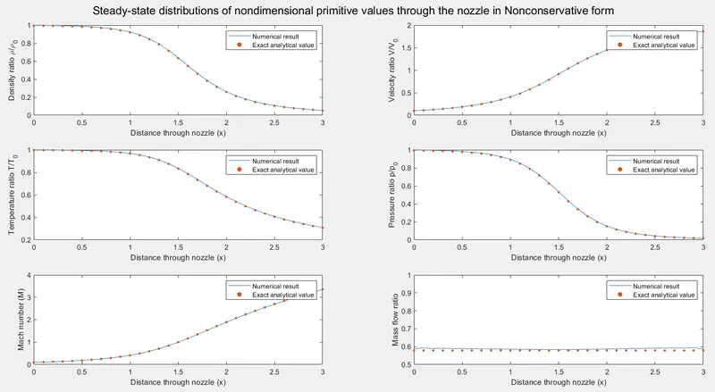
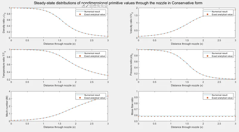
The comparisons show that numerical results agree very well with the exact analytical values. These are the results obtained after 1400 time steps.

2. Time-wise variation of the primitive variables

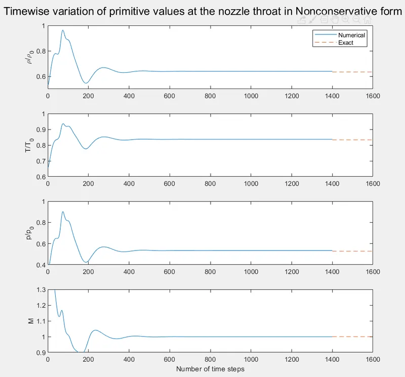
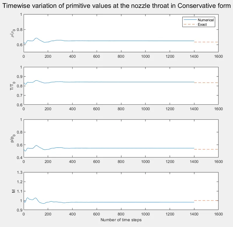
The graphs above show the variations of density, T, p y M ratios at the nozzle throat versus the number of time steps. The largest changes take place at early times and after time steps we can reach the steady state, it could be compared with the exact value (the dashed line in the graphs). The oscilations in the nonconservative form are larger at the first time steps than the conservative forms, because the initial conditions used in the conservative form are slightly more realistic. However, graphically we can see that the steady-state values obtained from the nonconservative seem to be nearier to the exact solution. It is one of the disadvantages of the conservative form.

3. Variation of Mass flow rate distribution inside the nozzle at different time steps during the time-marching process

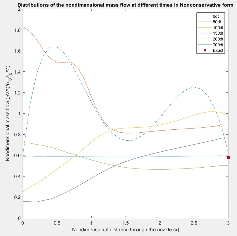
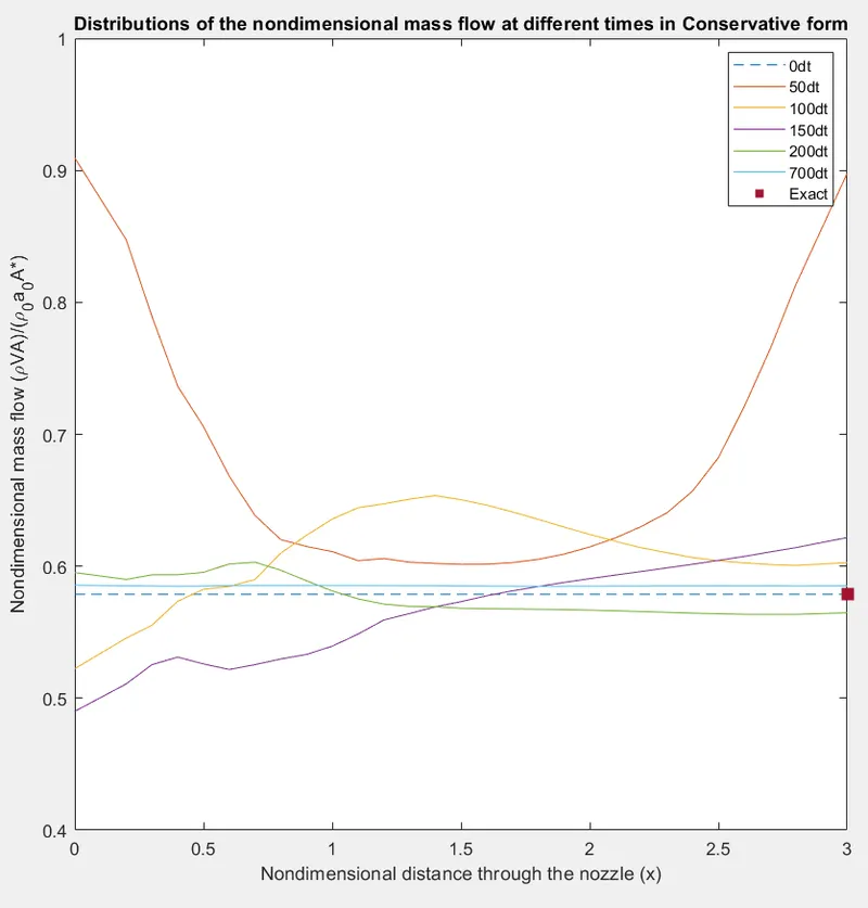
In regard to the variation of the mass flow ratio, the dashed curves are the variations of the mass flow ratio which belong to the initial conditions, we can see that the mass flow ratio in the conservative form is more accurate than the nonconservative form. The mass flow ratio variation is oscilating due to the transient variation of the flow field variables. Aftes approximately 700 time steps, the mass flow distribution is a horizontal line across the graph, this means that the mass flow ratio has converged to a constant, it agrees with the square in the graphs, which represents the constant value of the exact mass flow.

4. Comparison of Normalized mass flow rate distributions of both forms

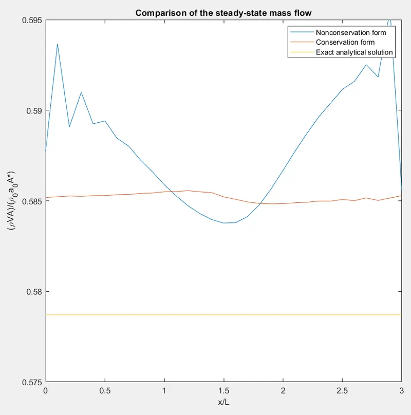
We can see that the steady-state mass flow distribution in the conservative form is more accurate than that obtained from the nonconservative form, because the mass flow is one of the dependent variables in the equations. The graph in noncoservative form has oscillations in the inflow and outflow boundaries. In fact, the distribution of the mass flow in conservative form is nearier to the exact distribution of the mass flow. This is one advantage of the conservative form.

Finally, we perform a grid independence test on the solution. The following code shows the comparisons of these values in a table. The results correspond to the throat of the nozzle.

clear all
close all
clc

%Inputs
L=3;
n_a=31;
n=[61 31];
nt=1400;
C=0.5;

%Solving the equation
%Analytical
[x,rho_a,v_a,T_a,p_a,M_a,m_a]=analytical_subsonic_supersonic_nozzle_function(L,n_a);
%Non conservative form
for i=1:2
    [x,rho_n{i},v_n,T_n{i},p_n{i},M_n{i},m_n,rho_throat_n,T_throat_n,p_throat_n,M_throat_n,m_time_n]=non_conservative_subsonic_supersonic_nozzle_function(L,n(i),nt,C);
end
%Conservative form
for j=1:2
    [x,rho_c{j},v_c,T_c{j},p_c{j},M_c{j},m_c,rho_throat_c,T_throat_c,p_throat_c,M_throat_c,m_time_c]=conservative_subsonic_supersonic_nozzle_function(L,n(j),nt,C);
end
fprintf('%6s %12s %10s %10s %10s %10s\n','Form','Points','rho/rho_o','T/T_o','p/p_o','M');
fprintf('%6s %12d %10.4f %10.4f %10.4f %10.4f\n','NC',n(1),rho_n{1}(31),T_n{1}(31),p_n{1}(31),M_n{1}(31));
fprintf('%6s %12d %10.4f %10.4f %10.4f %10.4f\n','NC',n(2),rho_n{2}(16),T_n{2}(16),p_n{2}(16),M_n{2}(16));
fprintf('%6s %12d %10.4f %10.4f %10.4f %10.4f\n','C',n(1),rho_c{1}(31),T_c{1}(31),p_c{1}(31),M_c{1}(31));
fprintf('%6s %12d %10.4f %10.4f %10.4f %10.4f\n','C',n(2),rho_c{2}(16),T_c{2}(16),p_c{2}(16),M_c{2}(16));
fprintf('%6s %12s %10.4f %10.4f %10.4f %10.4f\n','A','exact',rho_a(16),T_a(16),p_a(16),M_a(16));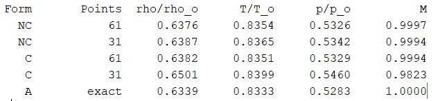  

Where NC is nonconservative, C is conservative and A is analytical.

Comparing the tho forms, the nonconservative form results are closer to the exact values. If we double the number of grid points (61 points) the numerical results are slightly closer to the exact analytical values. Also, both values (31 and 61 points) are almost the same, and we can say that using 31 points is grid independent.