Week 8 - Simulation of a backward facing step in OpenFOAM
The two cases is about a backward facing step.
The solvers folder was navigated at first. Because the flow described is incompressible-laminar viscous, the incompressible folder is chosen.

Inside this folder, the solver icoFoam is chosen because it describes the physics of the flow.

Next, inside the tutorials folder we choose the tutorials corresponding to icoFoam solver, finally we choose the cavity folder because it has the neccesary scripts and folders to this challenge.
Governing Equations
The Navier-Stokes equations (for a Newtonian fluid) are simplified since there are some considerations to do: the case is two dimensional, incompressible and ignore the source body force of gravity.
- Continuity equation:
Initially we have: `(delrho)/(delt)+nabla.(rho baru)=0`
Taking the considerations above, the equation is reduced to: `nabla.baru=0`
- Momentum equations:
The x-momentum equation is reduced to:
`(del rhou)/(delt)+nabla.(rhou.baru)=-(delp)/(delx)+(del)/(delx)(2mu(delu)/(delx))+(del)/(dely)(mu((delv)/(delx)+(delu)/(dely)))`
Let's reduce the viscous term:
`(del)/(delx)(mu(delu)/(delx))+(del)/(dely)(mu(delu)/(dely))+(del)/(delx)(mu(delu)/(delx))+(del)/(dely)(mu(delv)/(delx))`
The third and fourth terms have smaller contributions to the viscous stress so they are ignored (Versteeg Malalasekera, 2007).
The two first terms are factorized: `(del)/(delx)(mu(delu)/(delx))+(del)/(dely)(mu(delu)/(dely))=nabla.(mugradu)`
The y-momentum equation is analogous, if we join the two momentum equations, we obtain:
`rho(delbaru)/(delt)+rhonabla.(baru.baru)=-nablap+nabla.(mugradbaru)`
Density constant is divided in each term and we consider the kinematic pressure as: `p=p/rho`, and the kinematic viscosity: `nu=mu/rho`.
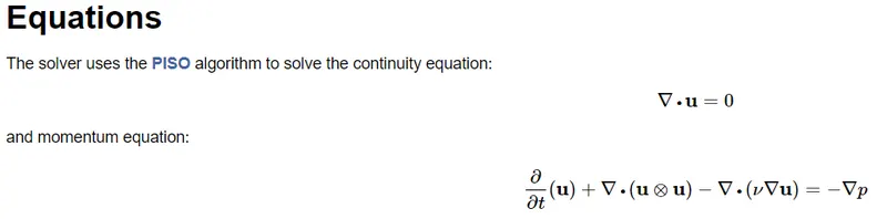
`(delbaru)/(delt)+nabla.(baru.baru)-nabla.(nugradbaru)=-nablap`
This equation has the same form as mentioned in the script of icoFoam.C
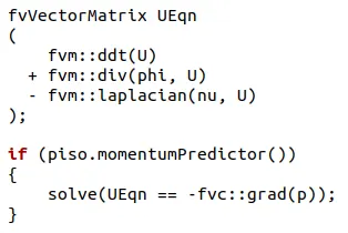
We can compare the obtained equations with the OpenFOAM: user guide - icoFoam.
Meshing the geometry with BlockMesh
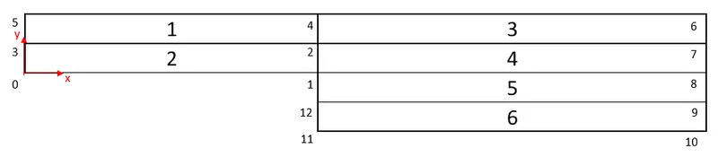
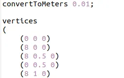
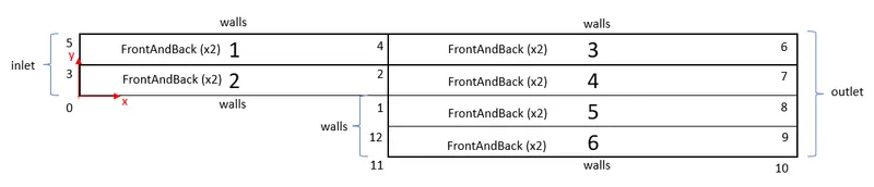
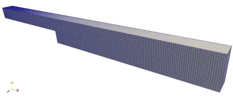
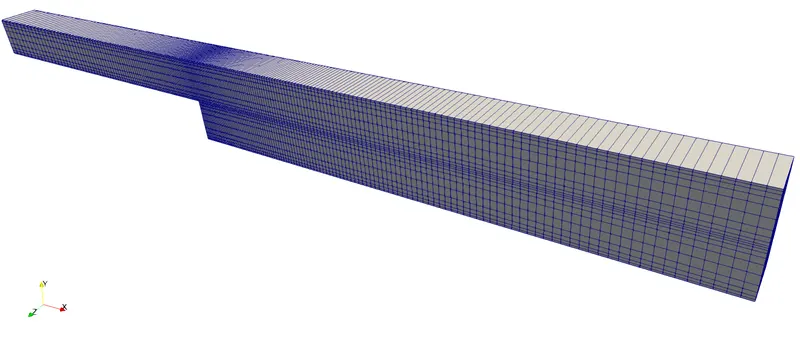
The geometry is divided in 6 blocks and the vertices are in the secuence that could be shown in the figures below.
- Back view:
- Front view:
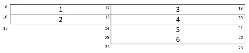
The vertices are put in "centimeters" for confort, then the note "convertToMeters 0.01" is implemented to obtain the distances like the assigment.
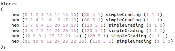
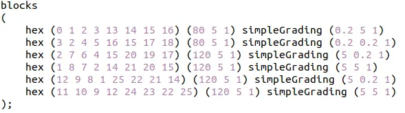
There are six blocks as I mentioned before, the difference between the two cases is here, because the grading factors are different.
The boundaries are called: inlet (2 faces), outlet (4 faces), walls (6 faces) and frontAndBack (12 faces).
The scripts of the two cases are the following.
Case 1:
/*--------------------------------*- C++ -*----------------------------------*\
  =========                 |
  \\      /  F ield         | OpenFOAM: The Open Source CFD Toolbox
   \\    /   O peration     | Website:  https://openfoam.org
    \\  /    A nd           | Version:  9
     \\/     M anipulation  |
\*---------------------------------------------------------------------------*/
FoamFile
{
    format      ascii;
    class       dictionary;
    object      blockMeshDict;
}
// * * * * * * * * * * * * * * * * * * * * * * * * * * * * * * * * * * * * * //

convertToMeters 0.01;

vertices
(
    (0 0 0)
    (8 0 0)
    (8 0.5 0)
    (0 0.5 0)
    (8 1 0)
    (0 1 0)
    (20 1 0)
    (20 0.5 0)
    (20 0 0)
    (20 -0.5 0)
    (20 -1 0)
    (8 -1 0)
    (8 -0.5 0)

    (0 0 1)
    (8 0 1)
    (8 0.5 1)
    (0 0.5 1)
    (8 1 1)
    (0 1 1)
    (20 1 1)
    (20 0.5 1)
    (20 0 1)
    (20 -0.5 1)
    (20 -1 1)
    (8 -1 1)
    (8 -0.5 1)
);

blocks
(
    hex (0 1 2 3 13 14 15 16) (80 5 1) simpleGrading (1 1 1)
    hex (3 2 4 5 16 15 17 18) (80 5 1) simpleGrading (1 1 1)
    hex (2 7 6 4 15 20 19 17) (120 5 1) simpleGrading (1 1 1)
    hex (1 8 7 2 14 21 20 15) (120 5 1) simpleGrading (1 1 1)
    hex (12 9 8 1 25 22 21 14) (120 5 1) simpleGrading (1 1 1)
    hex (11 10 9 12 24 23 22 25) (120 5 1) simpleGrading (1 1 1)
);

edges
(
);

boundary
(
    inlet
    {
        type wall;
        faces
        (
            (0 13 16 3)
            (3 16 18 5)

        );
    }
    outlet
    {
        type wall;
        faces
        (
            (7 6 19 20)
            (8 7 20 21)
            (9 8 21 22)
            (10 9 22 23)
        );
    }
    walls
    {
        type wall;
        faces
        (
            (4 5 18 17)
            (6 4 17 19)
            (11 10 23 24)
            (12 11 24 25)
            (1 12 25 14)
            (0 1 14 13)
        );
    }
    frontAndBack
    {
        type empty;
        faces
        (
            (0 3 2 1)
            (3 5 4 2)
            (2 4 6 7)
            (1 2 7 8)
            (12 1 8 9)
            (11 12 9 10)
            (13 14 15 16)
            (16 15 17 18)
            (15 20 19 17)
            (14 21 20 15)
            (25 22 21 14)
            (24 23 22 25)
        );
    }
);

mergePatchPairs
(
);

// ************************************************************************* //
Case 2:
/*--------------------------------*- C++ -*----------------------------------*\
  =========                 |
  \\      /  F ield         | OpenFOAM: The Open Source CFD Toolbox
   \\    /   O peration     | Website:  https://openfoam.org
    \\  /    A nd           | Version:  9
     \\/     M anipulation  |
\*---------------------------------------------------------------------------*/
FoamFile
{
    format      ascii;
    class       dictionary;
    object      blockMeshDict;
}
// * * * * * * * * * * * * * * * * * * * * * * * * * * * * * * * * * * * * * //

convertToMeters 0.01;

vertices
(
    (0 0 0)
    (8 0 0)
    (8 0.5 0)
    (0 0.5 0)
    (8 1 0)
    (0 1 0)
    (20 1 0)
    (20 0.5 0)
    (20 0 0)
    (20 -0.5 0)
    (20 -1 0)
    (8 -1 0)
    (8 -0.5 0)

    (0 0 1)
    (8 0 1)
    (8 0.5 1)
    (0 0.5 1)
    (8 1 1)
    (0 1 1)
    (20 1 1)
    (20 0.5 1)
    (20 0 1)
    (20 -0.5 1)
    (20 -1 1)
    (8 -1 1)
    (8 -0.5 1)
);

blocks
(
    hex (0 1 2 3 13 14 15 16) (80 5 1) simpleGrading (0.2 5 1)
    hex (3 2 4 5 16 15 17 18) (80 5 1) simpleGrading (0.2 0.2 1)
    hex (2 7 6 4 15 20 19 17) (120 5 1) simpleGrading (5 0.2 1)
    hex (1 8 7 2 14 21 20 15) (120 5 1) simpleGrading (5 5 1)
    hex (12 9 8 1 25 22 21 14) (120 5 1) simpleGrading (5 0.2 1)
    hex (11 10 9 12 24 23 22 25) (120 5 1) simpleGrading (5 5 1)
);

edges
(
);

boundary
(
    inlet
    {
        type wall;
        faces
        (
            (0 13 16 3)
            (3 16 18 5)

        );
    }
    outlet
    {
        type wall;
        faces
        (
            (7 6 19 20)
            (8 7 20 21)
            (9 8 21 22)
            (10 9 22 23)
        );
    }
    walls
    {
        type wall;
        faces
        (
            (4 5 18 17)
            (6 4 17 19)
            (11 10 23 24)
            (12 11 24 25)
            (1 12 25 14)
            (0 1 14 13)
        );
    }
    frontAndBack
    {
        type empty;
        faces
        (
            (0 3 2 1)
            (3 5 4 2)
            (2 4 6 7)
            (1 2 7 8)
            (12 1 8 9)
            (11 12 9 10)
            (13 14 15 16)
            (16 15 17 18)
            (15 20 19 17)
            (14 21 20 15)
            (25 22 21 14)
            (24 23 22 25)
        );
    }
);

mergePatchPairs
(
);

// ************************************************************************* //
We obtain the following graphs:
Case1:
Case2:
Reynolds number: We consider a initial velocity along x axis equal to 0.1 m/s and the kinematic viscosity of 0.0001, obtaining a Re = 10, because is a low value, it is laminar.
`Re=(uD)/(nu)=(0.1*0.01)/(0.0001)=10`
Courant number: This is stated by the formula (extracted from the OpenFOAM: User Guide - CourantNo)
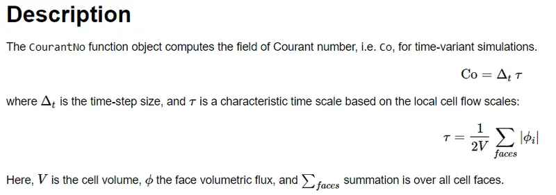
If we evaluate the Courant number in one cell of the inlet at the first time step, we assume at first Ux=1 m/s, dt=0.005 (from the case cavity), and dx=0.001. Then we obtain `Co=(dt.Ux)/(2*dx)=(0.005*1)/(2*0.001)=2.5`.
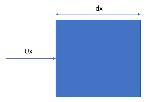
This value is large, as a consequence, the simulation was stopped. Then the Ux is reduced to 0.1 m/s so the value of Co is now 0.25. Hence the simulation was succeed.
Other modifications:
The scripts U and p in the folder 0 were modificated as follows:
/*--------------------------------*- C++ -*----------------------------------*\
  =========                 |
  \\      /  F ield         | OpenFOAM: The Open Source CFD Toolbox
   \\    /   O peration     | Website:  https://openfoam.org
    \\  /    A nd           | Version:  9
     \\/     M anipulation  |
\*---------------------------------------------------------------------------*/
FoamFile
{
    format      ascii;
    class       volVectorField;
    object      U;
}
// * * * * * * * * * * * * * * * * * * * * * * * * * * * * * * * * * * * * * //

dimensions      [0 1 -1 0 0 0 0];

internalField   uniform (0 0 0);

boundaryField
{
    inlet
    {
        type            fixedValue;
        value           uniform (0.1 0 0);
    }

    outlet
    {
        type            zeroGradient;
    }

    walls
    {
        type            noSlip;
    }

    frontAndBack
    {
        type            empty;
    }
}

// ************************************************************************* //
/*--------------------------------*- C++ -*----------------------------------*\
========= |
\\ / F ield | OpenFOAM: The Open Source CFD Toolbox
\\ / O peration | Website: https://openfoam.org
\\ / A nd | Version: 9
\\/ M anipulation |
\*---------------------------------------------------------------------------*/
FoamFile
{
format ascii;
class volScalarField;
object p;
}
// * * * * * * * * * * * * * * * * * * * * * * * * * * * * * * * * * * * * * //
dimensions [0 2 -2 0 0 0 0];
internalField uniform 0;
boundaryField
{
inlet
{
type zeroGradient;
}
outlet
{
type fixedValue;
value uniform 0;
}
walls
{
type zeroGradient;
}
frontAndBack
{
type empty;
}
}
// ************************************************************************* //In the script controlDict, the time was extended to 4.
Post-processing
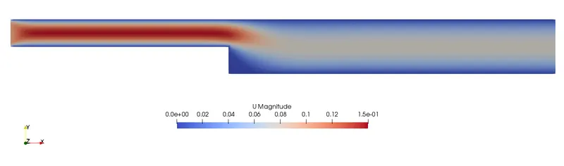
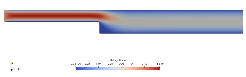
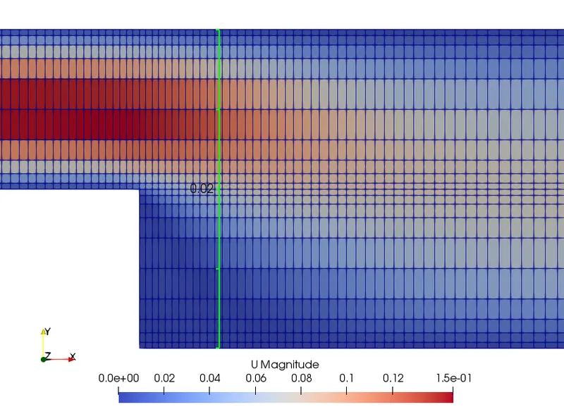
The plots in paraview are the following
Case1:
Case2:
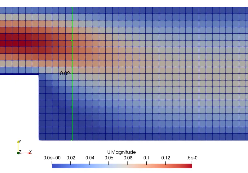
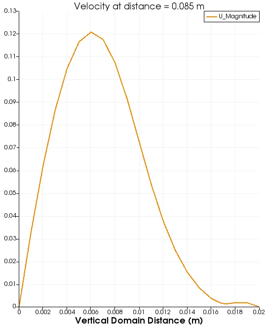
We use the option to plot using a line probe at x=0.085 m.
Case1:
Case2:
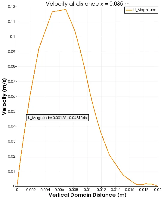
We export the data to Excel and graph both plots to compare.
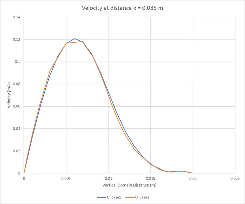
In the peak of the plots (the longest value of velocity) there are detailed results in the case1 because the mesh is finer. However, the results are slightly different between x=0.075 and x=0.015, the values in the case 2 should be more accurate because the mesh are finer, the same happens in the zones near to the walls. Because the viscosity effect near the walls, the mesh would be finer as the case 2, as a consequence, the results are more accurate and detailed.
Some extras:
The residuals were plot to verify this values and the relation with the number of iterations. This was for the case 1. After some commands, we obtain the following.
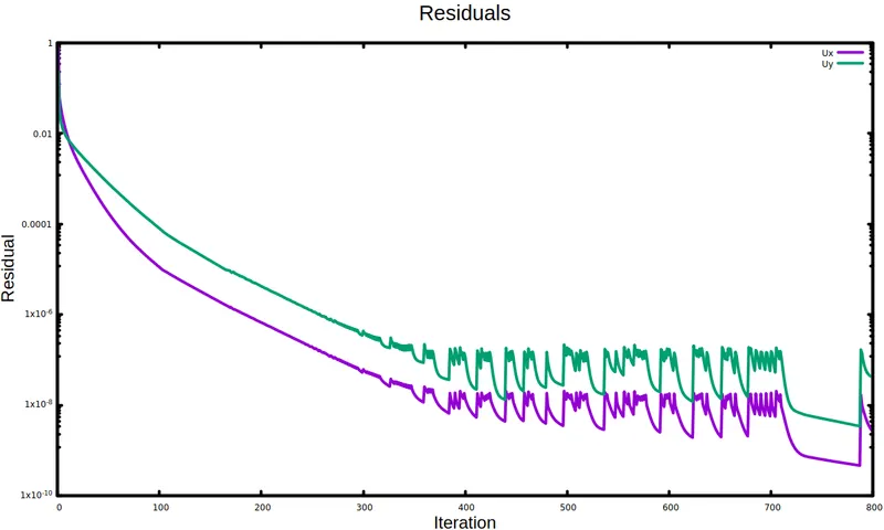
It seems that after 500 iterations the residuals are suffitiently low to have a "steady state" condition. It was in the order of approximately 1x10^-8.