Week 5.1 - Mid term project - Solving the steady and unsteady 2D heat conduction problem

This project consists in solve the steady and unsteady 2D heat conduction problem. They can be expressed mathematically in their differential form:

Steady equation:

`{del^2T}/{delx^2}+{del^2T}/{dely^2}=0`

Unsteady equation:

`{delT}/{delt}+alpha({del^2T}/{delx^2}+{del^2T}/{dely^2})=0`

where `T`is the dependent variable of temperature in the XY domain, `alpha` is the diffusion coefficient

1. Solving the steady state 2D heat conduction:

We can say that this equation is represented by the Laplace equation:

`{del^2phi}/{delx^2}+{del^2phi}/{dely^2}=0`

And this equation is known to has an elliptic nature, this means that a unique solution to this equation can be obtained by especifying conditions on the dependent variables (here the temperature) on all the boundaries of the solution domain. This type of problems are called boundary-value problems. Let's begin with the values os the boundary conditions for T.

Top Boundary = 600 K, Bottom Boundary = 900 K, Left Boundary = 400 K, Right Boundary = 800 K. It could be represented in this figure:

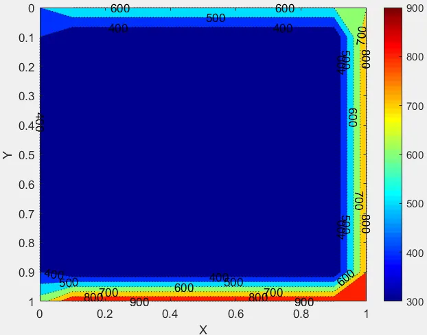
The values in the interior of the domain is defined as 300 K, it will be explained later. A code for the temperature field is implemented.

function T=T_initial_function(T_guess,nx,ny)
T=T_guess*ones(nx,ny); %Temperature in the interior of the domain
Ttop=600;
Tbottom=900;
Tleft=400;
Tright=800;
T(1,:)=Ttop;
T(end,:)=Tbottom;
T(:,1)=Tleft;
T(:,end)=Tright;
% Temperatures in the corners are averages
T(1,1)=0.5*(Ttop+Tleft);
T(1,end)=0.5*(Ttop+Tright);
T(end,1)=0.5*(Tbottom+Tleft);
T(end,end)=0.5*(Tbottom+Tright);
end

The finite difference method will be used to discretize the PDE. For the second derivatives terms, the central differencing scheme will be implemented because it takes information from the surroundings, and it ensures the elliptic nature.

 `{T_L-2T_P+T_R}/{trianglex^2}+{T_T-2T_P+T_B}/{triangley^2}=0`

`T_P={1}/{k}({T_L+T_R}/{trianglex^2})+{1}/{k}({T_T+T_B}/{triangley^2})`

where `k={2(trianglex^2+triangley^2)}/{trianglex^2triangley^2}`

Now, iterative solvers are implemented to obtain a solution. The iterative solver that will be used are Jacobi and Gauss-Seidel, they can be accelerated or decelerated by the SOR factor.

A code defined as the function that solve the steady equation and collect the both Jacobi and Gauss-Seidel is implemented

function out=steady_2d_heat_conduction_function(iterative_solver,w,x,y,nx,ny,dx,dy,T,tol)
error=9e9;
Told=T; %Told is the guess value for initial temperature field
k=2*(dx^2+dy^2)/(dx^2*dy^2);

%Jacobi method
if iterative_solver==1
    n_iter=1;
%Convergence loop
tic
while(error>tol)
    for i=2:nx-1
        for j=2:ny-1
            T(i,j)=1/(k*dx^2)*(Told(i-1,j)+Told(i+1,j))+1/(k*dy^2)*(Told(i,j-1)+Told(i,j+1));
            T(i,j)=(1-w)*Told(i,j)+w*(T(i,j));
        end
    end
    error=max(max(abs(Told-T)));
    Told=T;
    n_iter=n_iter+1;
end
time=toc;
meshgrid(x,y);
%Plotting temperature field
figure(1)
[X,Y]=contourf(x,y,T,':');
colormap(jet)
clabel(X,Y);
set(gca,'ydir','reverse')
if w>1
    title_text1=sprintf('SOR factor = %f (over-relaxation)',w);
elseif w<1
    title_text1=sprintf('SOR factor = %f (under-relaxation)',w);
else
    title_text1=sprintf('Without SOR factor');
end
title_text2=sprintf('Iteration number = %d',n_iter);
title_text3=sprintf('Iteration time = %f',time);
title({'Steady State 2D Heat Conduction';'Jacobi method';title_text1;title_text2;title_text3})
end

%Gauss-Seidel method
if iterative_solver==2
    n_iter=1;
%Convergence loop
tic
while(error>tol)
    for i=2:nx-1
        for j=2:ny-1
            T(i,j)=1/(k*dx^2)*(T(i-1,j)+Told(i+1,j))+1/(k*dy^2)*(T(i,j-1)+Told(i,j+1));
            T(i,j)=(1-w)*Told(i,j)+w*(T(i,j));
        end
    end
    error=max(max(abs(Told-T)));
    Told=T;
    n_iter=n_iter+1;
end
time=toc;
meshgrid(x,y);
%Plotting temperature field
figure(2)
[X,Y]=contourf(x,y,T,':');
colormap(jet)
clabel(X,Y);
set(gca,'ydir','reverse')
if w>1
    title_text1=sprintf('SOR factor = %f (over-relaxation)',w);
elseif w<1
    title_text1=sprintf('SOR factor = %f (under-relaxation)',w);
else
    title_text1=sprintf('Without SOR factor');
end
title_text2=sprintf('Iteration number = %d',n_iter);
title_text3=sprintf('Iteration time = %f',time);
title({'Steady State 2D Heat Conduction';'Gauss-Seidel method';title_text1;title_text2;title_text3})
end
out=n_iter;
end

The function display a plot of the converged results, the number and time (using the command tic toc on MatLAB) of iterations. Also this returns the number of iterations.

The following script allow to show the plot obtained from the prior function, and the inputs parameters can be defined. 

clear all
close all
clc

%Define inputs
Lx=1; %Length x
Ly=1; %Length y
nx=11; %number of nodes x axis
ny=11; %number of nodes y axis
tol=1e-4; %min tolerance for iterative solvers 

%Creating mesh
x=linspace(0,Lx,nx); 
y=linspace(0,Ly,ny);
dx=Lx/(nx-1);
dy=Ly/(ny-1);

%Define intial Temperature field
T_guess=300;
T=T_initial_function(T_guess,nx,ny);

%Numerical solutions

%First argument of the function:
%1=Jacobi solver, 2=Gauss-Seidel solver
%Second argument of the function: 
%SOR factor: w>1(over-relaxation), w<1(under-relaxation)

jacobi_iter=steady_2d_heat_conduction_function(1,1,x,y,nx,ny,dx,dy,T,tol);
gs_iter=steady_2d_heat_conduction_function(2,1,x,y,nx,ny,dx,dy,T,tol);
gs_SOR_iter=steady_2d_heat_conduction_function(2,1.5,x,y,nx,ny,dx,dy,T,tol);

Note that T_guess is the guess value of the temperature in the interior of the domain, this is required for the procedure of the iterations solvers. In this case: T_guess = 300 K.

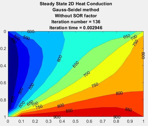
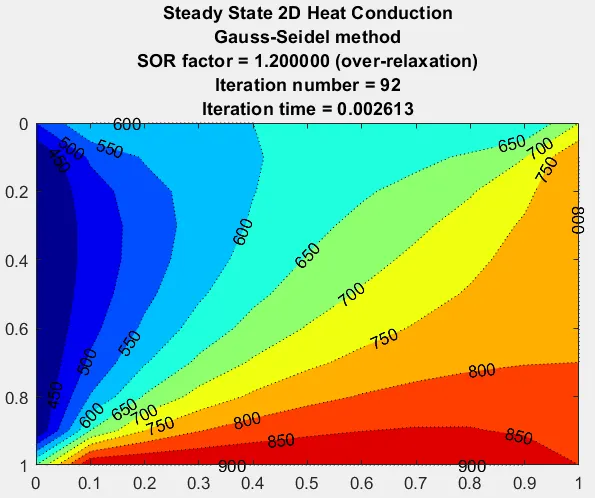
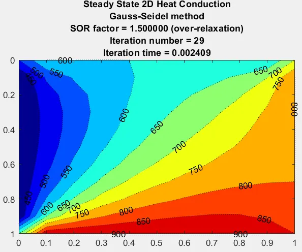
The plots obtained have this form:

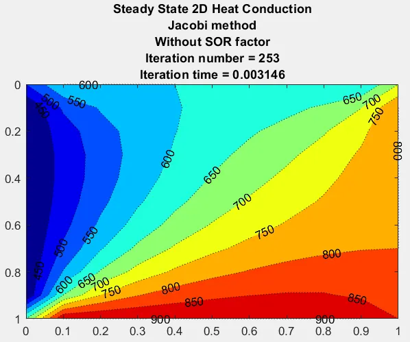
This iteration solvers are analysed and observations are the following:

• From the figures above, the Gauss-Seidel (G-S) method is more efficient because the number of iterations (136) is less than the obtained from the Jacobi method (253), as a result, it saves iteration's time (0.003146 for Jacobi, 0.002946 for G-S).
• The SOR factor accelerates the finding of the converged solution. In the case above, the factor is guess as 1.2 (over-relaxation) for the G-S method, and the number of iterations are 92 (less than 136 for G-S whitout the use of a SOR factor).
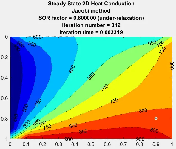
• If a SOR factor of 1.2 is implemented in the Jacobi method, a divergence in the solution wil occur, but it is not the case by the use of 0.8 of SOR factor (under-relaxation) for the same method, although the number of iterations is greater than the use of Jacobi method only.

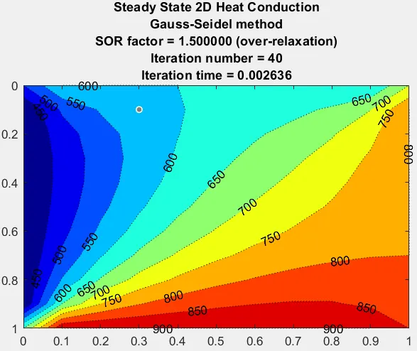
• Trying to find a SOR factor that save the number of iterations, and of course, save time, with the value of 1.5 or 1.6 in the G-S method, it is possible to obtain 40 iterations, values less than 1.5  or greater of 1.6 tend to increase the number of iterations, until even the case of divergence (value of 2 for SOR factor as an example).

• The cases above were obtained using 11 nodes in the X and Y domain. Of course, the increase of nodes results in the increment of iterations for both iterations solvers. Another parameter that influence on the converged solution is the guess value of the temperature as the initial value of iteration, that is 300 K. If the value is increased to 700 K, is possible to reduce the number of iterations. 

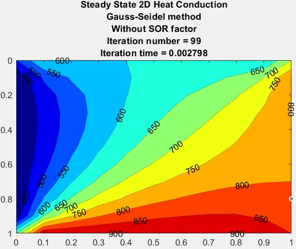
• Finally, if the SOR factor is added, it is possible to save more time. For example: T_guess = 800 K, SOR = 1.5, G-S method

2. Solving the unsteady state 2D heat conduction:

This equation is known to be parabolic, which describes time-dependent problems and involves significant amounts of diffusion. Here, all its boundaries are required for all times t>0 and intial conditions are needed in the entire domain. This type of problem is termed an initial-boundary-value-problem.

The solution moves forward in time an diffuse in space. The steady state is reached and is elliptic.

According to the definition above. The boundaries in all the times are termed: Top Boundary = 600 K, Bottom Boundary = 900 K, Left Boundary = 400 K, Right Boundary = 800 K. Also the initial conditions in all the domain will be the same as in section 1.

The finite difference method will be used to discretize the PDE. For the second derivatives terms, the central differencing scheme will be implemented and for the time derivative, the forward difference scheme will be used.

Explicit form:

 `{T_P^(n+1)-T_P^(n)}/{trianglet}=alpha({T_L-2T_P+T_R}/{trianglex^2}+{T_T-2T_P+T_B}/{triangley^2})^(n)`

Implicit form:

`{T_P^(n+1)-T_P^(n)}/{trianglet}=alpha({T_L-2T_P+T_R}/{trianglex^2}+{T_T-2T_P+T_B}/{triangley^2})^(n+1)`

 2.1. Solving the unsteady 2D heat conduction equation in explicit form:

 `{T_P^(n+1)-T_P^(n)}/{trianglet}=alpha({T_L-2T_P+T_R}/{trianglex^2}+{T_T-2T_P+T_B}/{triangley^2})^(n)`

`T_P^(n+1)=T_P^(n)+k_1(T_L-2T_P+T_R)^n+k_2(T_T-2T_P+T_B)^n`

 where `k_1=alpha{trianglet}/{trianglex^2}` and `k_2=alpha{trianglet}/{triangley^2}`

A diffusion stability condition will be defined as follow:

`CFL_x=k_1` and `CFL_y=k_2`

`CFL_x+CFL_y<0.5`the solution tend to converge.

A code defined as the function that solve the unsteady equation. Note that iterative solvers are not used because the explicit form solves the system directly. Moreover, the values in the right hand side are known.

function out=unsteady_2d_heat_conduction_explicit_function(x,y,nx,ny,nt,k1,k2,T)
Told=T;
%Time loop
tic
for k=1:nt
    %Space loop
    for i=2:nx-1
        for j=2:ny-1
            T(i,j)=(1-2*k1-2*k2)*Told(i,j)+k1*(Told(i-1,j)+Told(i+1,j))+k2*(Told(i,j-1)+Told(i,j+1));
        end
    end
    %Update temperatures
    Told=T;
end
time=toc;
out=time;
%Plot temperatures
%meshgrid(x,y);
[X,Y]=contourf(x,y,T,':');
colormap(jet)
clabel(X,Y)
set(gca,'ydir','reverse')
title_text=sprintf('Iteration time = %f',time);
title({'Unsteady State 2D Heat Conduction';'Explicit form';title_text})
end

 The function display a plot of the converged results and the time (using the command tic toc on MatLAB) of iterations. Also this returns the time of iterations.

2.2. Solving the unsteady 2D heat conduction equation in implicit form:

`{T_P^(n+1)-T_P^(n)}/{trianglet}=alpha({T_L-2T_P+T_R}/{trianglex^2}+{T_T-2T_P+T_B}/{triangley^2})^(n+1)`

`T_P^(n+1)(1+2k_1+2k_2)=T_P^(n)+k_1(T_L+T_R)^(n+1)+k_2(T_T+T_B)^(n+1)`

`term1={1}/{1+2k_1+2k_2}`

`term2=term1*k_1`

`term3=term1*k_2`

`T_P^(n+1)=term1*T_P^(n)+term2(T_L+T_R)^(n+1)+term3(T_T+T_B)^(n+1)`

A code defined as the function that solve the unsteady equation. Note that iterative solvers are used because the unknown values in the right hand side become the algebraic equations in a system of equations.

function out=unsteady_2d_heat_conduction_implicit_function(iterative_solver,w,x,y,nx,ny,nt,k1,k2,T,tol)
Told=T;
T_prev=T;

%Jacobi method
if iterative_solver==1
%Time loop 
tic
for k=1:nt
    error=9e9;
    %Convergence loop
    while (error>tol)
        for i=2:nx-1
            for j=2:ny-1
                %Jacobi
                term1=1/(1+2*k1+2*k2);
                term2=k1*term1;
                term3=k2*term1;
                H=Told(i-1,j)+Told(i+1,j);
                V=Told(i,j-1)+Told(i,j+1);
                T(i,j)=T_prev(i,j)*term1+H*term2+V*term3;
                T(i,j)=(1-w)*Told(i,j)+w*(T(i,j));
            end
        end
        error=max(max(abs(Told-T)));
        Told=T;
    end
    T_prev=T;
end
time=toc;
meshgrid(x,y);
%Plotting temperature field
figure(1)
[X,Y]=contourf(x,y,T,':');
colormap(jet)
clabel(X,Y);
set(gca,'ydir','reverse')
xlabel('X')
ylabel('Y')
if w>1
    title_text1=sprintf('SOR factor = %f (over-relaxation)',w);
elseif w<1
    title_text1=sprintf('SOR factor = %f (under-relaxation)',w);
else
    title_text1=sprintf('Without SOR factor');
end
title_text2=sprintf('Iteration time = %f',time);
title({'Unsteady State 2D Heat Conduction';'Jacobi method';title_text1;title_text2})
end

%Gauss-Seidel method
if iterative_solver==2
%Time loop 
tic
for k=1:nt
    error=9e9;
    %Convergence loop
    while (error>tol)
        for i=2:nx-1
            for j=2:ny-1
                %Jacobi
                term1=1/(1+2*k1+2*k2);
                term2=k1*term1;
                term3=k2*term1;
                H=T(i-1,j)+Told(i+1,j);
                V=T(i,j-1)+Told(i,j+1);
                T(i,j)=T_prev(i,j)*term1+H*term2+V*term3;
                T(i,j)=(1-w)*Told(i,j)+w*(T(i,j));
            end
        end
        error=max(max(abs(Told-T)));
        Told=T;
    end
    T_prev=T;
end
time=toc;
meshgrid(x,y);
%Plotting temperature field
figure(2)
[X,Y]=contourf(x,y,T,':');
colormap(jet)
clabel(X,Y);
set(gca,'ydir','reverse')
xlabel('X')
ylabel('Y')
if w>1
    title_text1=sprintf('SOR factor = %f (over-relaxation)',w);
elseif w<1
    title_text1=sprintf('SOR factor = %f (under-relaxation)',w);
else
    title_text1=sprintf('Without SOR factor');
end
title_text2=sprintf('Iteration time = %f',time);
title({'Unsteady State 2D Heat Conduction';'Gauss-Seidel method';title_text1;title_text2})
end
out=time;
end

 The function display a plot of the converged results and the time (using the command tic toc on MatLAB) of iterations. Also this returns the time of iterations and the method that is used.

The following script allow to show the plot obtained from the prior functions (explicit and implicit), and the inputs parameters can be defined. 

clear all
close all
clc

%Define inputs
Lx=1; %Length x
Ly=1; %Length y
nx=11; %number of nodes x axis
ny=11; %number of nodes y axis
alpha=1.4; %diffusion coefficient
dt=1e-3;
nt=1.4/dt;
tol=1e-4; %min tolerance for iterative solvers 

%Creating mesh
x=linspace(0,Lx,nx);
y=linspace(0,Ly,ny);
dx=Lx/(nx-1);
dy=Ly/(ny-1);

%Define intial Temperature field
T=T_initial_function(300,nx,ny);

%CFL values
k1=alpha*dt/(dx^2);
k2=alpha*dt/(dy^2);
CFL=k1+k2

%Numerical Solutions

%Explicit form
time_explicit=unsteady_2d_heat_conduction_explicit_function(x,y,nx,ny,nt,k1,k2,T)

%Implicit form
%First argument of the function:
%1=Jacobi solver, 2=Gauss-Seidel solver
%Second argument of the function: 
%SOR factor: w>1(over-relaxation), w<1(under-relaxation)
time_implicit_Jacobi=unsteady_2d_heat_conduction_implicit_function(1,1,x,y,nx,ny,nt,k1,k2,T,tol)
time_implicit_Jacobi_SOR=unsteady_2d_heat_conduction_implicit_function(1,1.2,x,y,nx,ny,nt,k1,k2,T,tol)
time_implicit_GS=unsteady_2d_heat_conduction_implicit_function(2,1,x,y,nx,ny,nt,k1,k2,T,tol)
time_implicit_GS_SOR=unsteady_2d_heat_conduction_implicit_function(2,1.1,x,y,nx,ny,nt,k1,k2,T,tol)

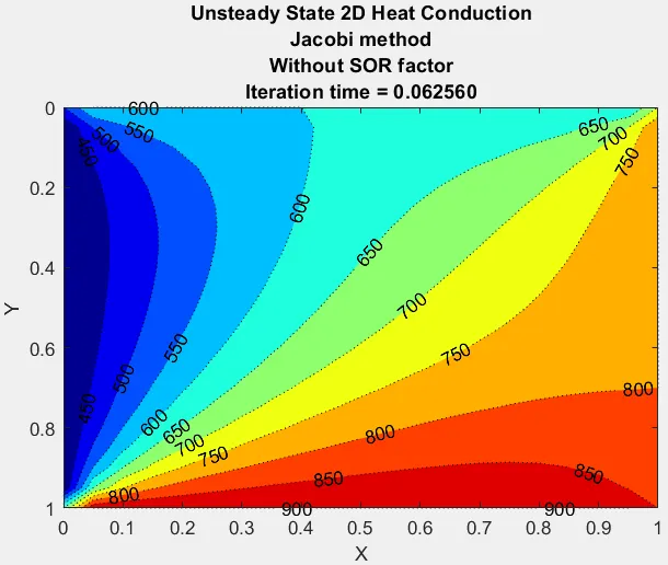
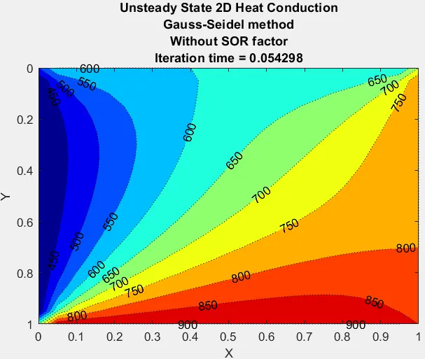
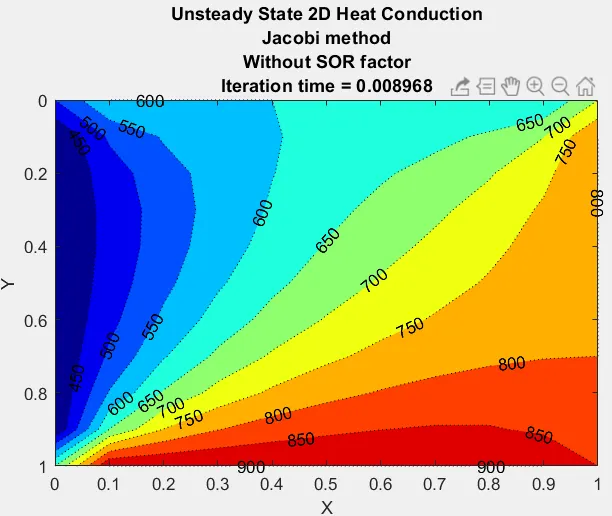
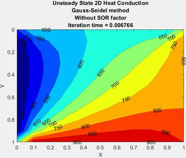
The plots obtained have this form:

 

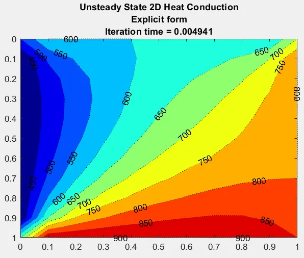
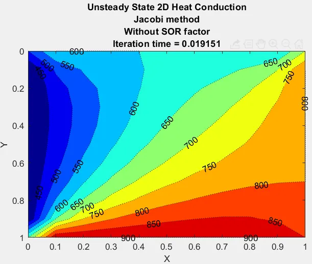
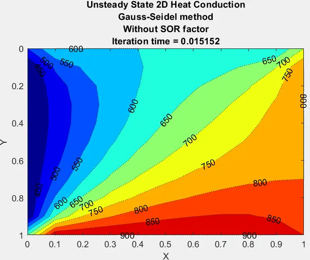
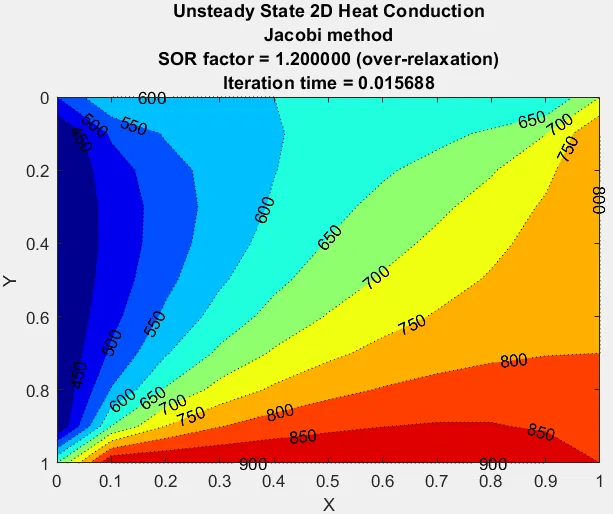
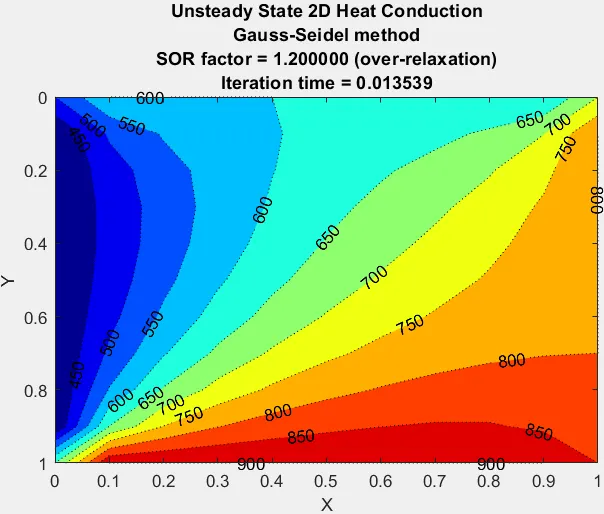
Observations of the results are the following:

The value of the CFL of the script above is 0.28 with the number of nodes `nx=ny=11`, `alpha=1.4` and `trianglet=1e-3`, this values is less than 0.5. Note that this condition is acceptable for explicit forms. If we decrease dx or dy (as a consequence of increase the number of nodes, for example), or maybe increment dt, the CFL factor then tends to increase and this becomes in an instability of the solution.

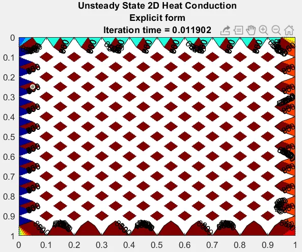
Of course, the solution with the Jacobi method take more time to converge, compared to the Gauss-Seidel. This could be shown in the figures above (the values of the time of iterations).

The `CFL<0.5` condition doesn't accomplish with the implicit method. For example, if we change the value of `trianglet=1e-2`, the value of `CFL=2.8>0.5`. The problem converges for the Jacobi and Gauss-Seidel method.

With the increase of nodes, 21 for example, `CFL=1.12>0.5`, but the problem converge too.