Week 3.5 - Deriving 4th order approximation of a 2nd order derivative using Taylor Table method

DERIVING THE FOLLOWING 4TH ORDER APPROXIMATIONS OF THE SECOND-ORDER DERIVATIVE.

1. Central difference.

We have the order of accuracy P = 4, the order of derivative Q = 2 for central schemes, so from the equation of the Hint, we obtain the number of nodes in the stencil N:

`P=N-Q+1`

`N=5`

We provide the following nodes: (i-2) (i-1) (i) (i+1) (i+2), each one separated by `Deltax`

The hipothesis function has the following form:

`(d^2u)/(dx^2)=af(i-2)+bf(i-1)+cf(i)+df(i+1)+ef(i+2)`

The matrix form of the Taylor table method is:

`[[1,1,1,1,1],[-2, -1, 0, 1, 2],[2 ,1/2, 0 ,1/2 ,2],[-8/6 ,-1/6, 0, 1/6, 8/6],[16/24, 1/24, 0 ,1/24 ,16/24]]((a),(b),(c),(d),(e))=((0),(0),(1),(0),(0))`

Solving the system of equations we obtain the coefficients:

`((a),(b),(c),(d),(e))=((-0.0833),(1.333),(-2.5),(1.333),(-0.0833))`

Now we get the fourth order central difference approximation:

`(d^2u)/(dx^2)=(-0.0833f(i-2)+1.3333f(i-1)-2.5000f(i)+1.3333f(i+1)-0.0833f(i+2))/(Deltax^2)`

2. Skewed right-sided difference.

We have the order of accuracy P = 4, the order of derivative Q = 2 for skewed schemes, so from the equation of the Hint, we obtain the number of nodes in the stencil N:

`P=N-Q`

`N=6`

We provide the following nodes: (i) (i+1) (i+2) (i+3) (i+4) (i+5), each one separated by `Deltax`

The hipothesis function has the following form:

`(d^2u)/(dx^2)=af(i)+bf(i+1)+cf(i+2)+df(i+3)+ef(i+4)+gf(i+5)`

The matrix form of the Taylor table method is:

`[[1,1,1,1,1,1],[0, 1, 2, 3, 4,5],[0 ,1/2 ,4/2 ,9/2 ,16/2 ,25/2],[0 ,1/6 ,8/6 ,27/6, 64/6 ,125/6],[0 ,1/24 ,16/24 ,81/24 ,256/24, 625/24],[0 ,1/120, 32/120, 243/120, 1024/120, 3125/120]]((a),(b),(c),(d),(e),(g))=((0),(0),(1),(0),(0),(0))`

Solving the system of equations we obtain the coefficients:

`((a),(b),(c),(d),(e),(g))=((3.7500),(-12.8333),(17.8333),(-13.0000),(5.0833),(-0.8333))`

Now we get the fourth order skewed right-sided difference approximation:

`(d^2u)/(dx^2)=(3.7500f(i)-12.8333f(i+1)+17.8333f(i+2)-13.0000f(i+3)+5.0833f(i+4)-0.8333f(i+5))/(Deltax^2)`

3. Skewed left-sided difference

We have the order of accuracy P = 4, the order of derivative Q = 2 for skewed schemes, so from the equation of the Hint, we obtain the number of nodes in the stencil N:

`P=N-Q`

`N=6`

We provide the following nodes: (i-5) (i-4) (i-3) (i-2) (i-1) (i), each one separated by `Deltax`

The hipothesis function has the following form:

`(d^2u)/(dx^2)=af(i-5)+bf(i-4)+cf(i-3)+df(i-2)+ef(i-1)+gf(i)`

The matrix form of the Taylor table method is:

`[[1,1,1,1,1,1],[-5, -4 ,-3, -2 ,-1 ,0],[25/2 ,16/2, 9/2 ,4/2 ,1/2, 0],[-125/6, -64/6 ,-27/6, -8/6, -1/6 ,0],[625/24 ,256/24 ,81/24 ,16/24, 1/24, 0],[-3125/120, -1024/120, -243/120 ,-32/120 ,-1/120, 0]]((a),(b),(c),(d),(e),(g))=((0),(0),(1),(0),(0),(0))`

Solving the system of equations we obtain the coefficients:

`((a),(b),(c),(d),(e),(g))=((-0.8333),(5.0833),(-13.0000),(17.8333),(-12.8333),(3.7500))`

Now we get the fourth order skewed right-sided difference approximation:

`(d^2u)/(dx^2)=(-0.8333f(i-5)+5.0833f(i-4)-13.0000f(i-3)+17.8333f(i-2)-12.8333f(i-1)+3.7500f(i))/(Deltax^2)`

PROGRAMMING IN MATLAB

We have the following function:

`f(x)=e^x*cos(x)`

Analytical derivative:

`f''(x)=-2*e^x*sin(x)`

Creating a function that return the dependent value of the function `f(x)=e^x*cos(x)`:

%Function
function y=f_x(x)
y=exp(x).*cos(x);
end

Creating a function that return the 4th order error of the central difference approximation:

function out=fourth_order_error_cds(x,dx)
second_derivative=-2*exp(x)*sin(x);
A_CDS=[1 1 1 1 1;
    -2 -1 0 1 2;
    2 1/2 0 1/2 2;
    -8/6 -1/6 0 1/6 8/6;
    16/24 1/24 0 1/24 16/24];
B_CDS=[0;0;1;0;0];
R_CDS=A_CDS\B_CDS;
fourth_order_approx_cds=(R_CDS(1)*f_x(x-2*dx)+R_CDS(2)*f_x(x-dx)+R_CDS(3)*f_x(x)+R_CDS(4)*f_x(x+dx)+R_CDS(5)*f_x(x+2*dx))./(dx.^2);
out=abs(second_derivative-fourth_order_approx_cds);
end

Creating a function that return the 4th order error of the skewed right-sided difference approximation:

function out=fourth_order_error_srd(x,dx)
second_derivative=-2*exp(x)*sin(x);
A_SRD=[1 1 1 1 1 1;
    0 1 2 3 4 5;
    0 1/2 4/2 9/2 16/2 25/2;
    0 1/6 8/6 27/6 64/6 125/6;
    0 1/24 16/24 81/24 256/24 625/24;
    0 1/120 32/120 243/120 1024/120 3125/120];
B_SRD=[0;0;1;0;0;0];
R_SRD=A_SRD\B_SRD;
fourth_order_approx_srd=(R_SRD(1)*f_x(x)+R_SRD(2)*f_x(x+dx)+R_SRD(3)*f_x(x+2*dx)+R_SRD(4)*f_x(x+3*dx)+R_SRD(5)*f_x(x+4*dx)+R_SRD(6)*f_x(x+5*dx))./(dx.^2);
out=abs(second_derivative-fourth_order_approx_srd);
end

Creating a function that return the 4th order error of the skewed left-sided difference approximation:

function out=fourth_order_error_sld(x,dx)
second_derivative=-2*exp(x)*sin(x);
A_SLD=[1 1 1 1 1 1;
    -5 -4 -3 -2 -1 0;
    25/2 16/2 9/2 4/2 1/2 0;
    -125/6 -64/6 -27/6 -8/6 -1/6 0;
    625/24 256/24 81/24 16/24 1/24 0;
    -3125/120 -1024/120 -243/120 -32/120 -1/120 0];
B_SLD=[0;0;1;0;0;0];
R_SLD=A_SLD\B_SLD;
fourth_order_approx_sld=(R_SLD(1)*f_x(x-5*dx)+R_SLD(2)*f_x(x-4*dx)+R_SLD(3)*f_x(x-3*dx)+R_SLD(4)*f_x(x-2*dx)+R_SLD(5)*f_x(x-dx)+R_SLD(6)*f_x(x))./(dx.^2);
out=abs(second_derivative-fourth_order_approx_sld);
end

Note: we use the coefficients of each matrix directly in the numerical approximation statements to avoid input errors.

Now we create a script that compare the absolute error between the above-mentioned schemes. we use the functions created above.

clear all
close all
clc
%Analytical function f(x)=exp(x)*cos(x)
%set values
x=pi/3;
dx=linspace(pi/40,pi/40000,80);

%Plotting
loglog(dx,fourth_order_error_cds(x,dx))
hold on
loglog(dx,fourth_order_error_srd(x,dx),'r')
hold on
loglog(dx,fourth_order_error_sld(x,dx),'g')
xlabel('Range dx')
ylabel('4th order Truncation Error')
legend('Central Difference Error','Skewed Right-sided Difference Error','Skewed Left-sided Difference Error')

Results:

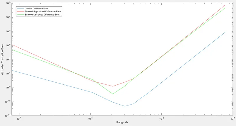
In the plot, we observe that the central difference approximation has less error than the others, although the skewed difference schemes take information of 5 points compared to the central difference that take information of 4 points from the surroundings.

We answer the question:

In your own words, describe why a skewed scheme is useful? What can a skewed scheme do that a CD scheme cannot?

The skewed scheme is useful when we want to solve the approximation in the boundaries, because we have to take the information from one side instead of central difference approximation, which we can take information from the surroundings.