Week 9 - FVM Literature Review

FVM LITERATURE

FINITE VOLUME METHOD:

The finite volume method (FVM) is a method for representing and evaluating partial differential equation in the form of algebraic equations. In the finite volume method, volume integrals in a partial differential equation that contain a divergence term are converted to surface integrals, using the divergence theorem. These terms are then evaluated as fluxes at the surfaces of each finite volume. Because the flux entering a given volume is identical to that leaving the adjacent volume, these methods are conservative. Another advantage of finite volume method is that it is easily formulated to allow for unstructured meshes. The method is used in many CFD packages.”Finite Volume “ refers to the small volume surrounding each node point on a mesh.

DIFFERENCE BETWEEN FVM AND FDM:

Finite difference method:

• The finite difference method is the most direct approach to discretizing based upon the differential form of the PDE to be solved. We consider a point in a space where we take the continuum representation of the equations and replace it with set discrete equations, called finite-difference equations.
• Boundary conditions are needed to truncate the computational domain. They represent communication with the surrounding world, which is the part that we do not want included in our simulation. With the finite-difference method, we may easily run into problems handling boundaries for the purpose of defining the boundary conditions.
• The finite-difference method is typically defined on a regular/structured grid and this fact can be used for very efficient solution methods. Regular grids are useful for very-large-scale simulations on supercomputers.
• This method is therefore not usually used for irregular CAD geometries, but more often for rectangular or block-shaped models.
• The finite-difference method is more difficult to use for handling material discontinuities. In addition, it does not lend itself for local grid refinement or anything similar to “adaptive mesh refinement”. This may be needed to resolve local rapid variations in solutions such as around a corner of a complex shape, as described earlier. But if we can fit the simulation in a rectangular or box-shaped geometry using a regular grid, efficient implementations are much easier than for finite- volume methods.
• If one can overcome the boundary-condition problem on curved boundaries, the method gives very efficient and high-quality results.
• The finite-difference method is defined dimension per dimension; this makes it easy to increase the “element order” to get higher-order accuracy.

Finite volume method:

• The finite-volume method is similar to the finite-differencing method in that the CAD model is first divided into very small but finite-sized elements of geometrically simple shapes. Apart from this, the finite-volume method is very different from the finite-differencing method, beginning with the concept of elements, which are instead referred to as cells.
• A finite volume method discretization is based upon as integral form of the PDE to be solved and can handle discontinuities in solutions. The PDE is written in a form which can be solved for a given finite volume. The computational domain is discretized into finite volumes and then for every volume the governing equations are solved. The resulting system of equations usually involves fluxes of the conserved variable, and thus the calculation of fluxes is very important in FVM.
• The finite-volume methods strength is that it only needs to do flux evaluation for the cell boundaries. This also holds for non-linear problems, which makes it extra powerful for robust handling of conservation laws appearing in transport problems.
• The local accuracy of the finite-volume method, such as close to a corner of interest, can be increased by refining the mesh around that corner. However, the functions that approximate the solution when using the finite-volume method cannot be easily made of higher order. This is a disadvantage of finite-volume method compared to the finite-difference method.
• The basic advantage of this method over FDM is it does not require the use of structured grids, and the effort to convert the given mesh in to structured numerical grid internally is completely avoided. As with FDM, the resulting approximate solution is a discrete, but the variables are typically placed at cell centre’s rather than at nodal points. This is not always true, as there are also face-centered finite volume methods. In any case, the values of filed variables at non-storage locations are obtained using interpolation.
• FVM can guarantee the local and global conservation of the system.

INTERPOLATION SCHEMES:

The approximations of surface and volume integrals require values of the variable at location other than the computational nodes of the control volume, Values at these locations are obtained using interpolation formulae.

Interpolation methods:

1. Upwind interpolation
2. Linear interpolation
3. Quadratic upwind interpolation
4. Hybrid, TVD and ENO interpolation schemes

Upwind Interpolation Scheme:

• It is mainly used for the convection dominant problems. Velocity for a given point, the direction of that particular velocity that determines the variables value used in interpolation process. Upwind scheme make use of nodes that are in the upstream of the given node.
• It is used to calculate the approximate value of the variable (f) at the east face of the control volume; the equation is given by

`f_e={[f_P if (V.n)_e>0],[f_E if (V.n)_e<0]}`

Where `f_P` is the point to the left of face e

`f_E` is the point to the right of face e

`V.n` is velocity vector

• This Scheme is almost similar to the forward difference approximation or backward difference approximation based on the flow direction.
• We know that, when calculating gradient, we need to have those values bounded, so that they don’t jump. Hence this approximation satisfies the boundless condition.

Linear Interpolation Scheme:

• Linear interpolation is the method of generating new data points with a range of discrete set of known data points.

`f_e=f_Elamda_e+f_P(1-lamda_e)`

Where,

`lamda_e=(x_e-x_P)/(x_E-x_p)`

• The linear interpolation scheme is same as the central difference formula that we considered for the first order derivative. So this scheme is also known as the central difference scheme.
• Generally it is used to solve the integrated convection-diffusion equation.
• It leads to an easy approximation for the evaluation of gradients that are required for evaluation of gradients that are required for evaluation of diffusive fluxes.
• CDS is a second order accurate and may produce oscillatory solutions i.e, here if the grid spacing is very large we can find oscillatory solutions. It is basically a first order, as we refine the grid then accuracy is close to the second order.

Quadratic upwind Interpolation Scheme:

• In CFD it is called as QUICK i.e, Quadratic Upstream Interpolation for convective kinematics.
• QUICK considers the second order derivative term into consideration and ignores the third order derivative term. Hence it is considered as third order accurate.
• Now approximate the value of the particular variable at the face centre of the control volume by the quadratic interpolation by using the values at three nearest computational nodes i.e, 1 downstream node(D) and two upstream (U,UU) respectively. The equation is given by;

`f_e=f_U+g_1(f_D-f_U)+g_2(f_(UU)-f_U)`

Where,

`g_1=((x_e-x_U)(x_e-x_(UU)))/(((x_D-x_U)(x_D-x_(UU))`

`g_2=((x_e-x_U)(x_e-x_(D)))/((x_(UU)-x_U)(x_(UU)-x_(D))`

• This scheme generally used to solve the convective-diffusion equations using the second order central difference for the diffusion term and for the convection term the scheme is third order accurate in space and first order accurate in time.

Hybrid Interpolation Scheme:

The hybrid difference scheme is a combination of the central difference scheme and upward difference scheme. It makes use of the central difference scheme, which is second-order accurate, for small Peclet numbers. For large Peclet numbers it uses the upwind difference scheme, which is first-order accurate but takes into account the convection of the fluid.

`f_e=gammaf_(CDS)+(1-gamma)f_(UDS)`

Total Variation Diminish Interpolation Scheme:

TVD scheme is employed to capture sharper shock predictions without any misleading oscillations when the variation of the field variables is discontinuous. To capture the variation fine grids are needed and the computation becomes heavy and therefore uneconomic. The use of coarse grids with CDS, upwind scheme, hybrid difference scheme gives false shock predictions. TVD scheme enables sharper shock predictions on coarse grids saving computation time and as the scheme preserves monotonicity there are no spurious oscillations in the solution.

`phi_(face)=6/8phi_(i-1)+3/8phi_i-1/8phi_(i-2)`

Where phi is flow property

FLUX LIMITER:

Flux limiters are used in high-resolution schemes i.e numerical schemes used to solve the problem in science and engineering, particularly fluid dynamics, described by PDE. They are used in high-resolution schemes, such as the MUSL scheme, to avoid the spurious oscillations that would otherwise occur with high order spatial discretization schemes due to shocks, discontinuities or sharp changes in the solution domain. The use of flux limiters, together with an appropriate high-resolution scheme, makes the solution total variation diminishing (TVD).

Note that flux limiters are also referred to as slope limiters, because they both have the same mathematical form and both have effect of limiting the solution gradient near shocks or discontinuities. In general, the term flux limiter acts on system states.

Need for Interpolation schemes and flux limiters in FVM

1. The Gauss divergence theorem simply states that the outward flux of a vector field through a closed surface is equal to the volume integral of the divergence over th region inside the surface.
2. This theorem is fundamental in the FVM; it is used to convert the volume integrals appearing in the governing equation into surface integrals.
3. The face values appearing in the convective and diffusive fluxes have to be computed by some form of interpolation from the centroid values of the control volume at both sides of the face.
4. After spatial discretization, we can proceed with the temporal discretization. By proceeding in this way we are using the method of lines (MOL).
5. The main advantage of the MOL method is that it allows us to select numerical approximations of different accuracy for the spatial and temporal terms. Each term can be treated differently to yield different accuracies.

EXAMPLE:

One dimensional steady state heat conduction:

Consider steady state diffusion of a property in one-demensional domain defined in the figure below. The process is governed by

`del/(delx)((Gammadelphi)/(delx))+S=0`

Finite Difference Method:

In finite difference method the total domain is discretized into grids .

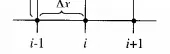
Later the discretization is done by three different interpolation schemes namely forward , backward and central differencing schemes.Based upon the problem the above mentioned schemes .We also use jacobi or gauss -sidel or SOR method to fasten the process and obtain at solution in minimal number of iterations

`(del^2phi)/(delx^2)=(phi_(i+1)^n-2phi_i^n+phi_(i-1)^n)/(Deltax^2)`

Later using this decretized form the solution for the equation is obtained by running the program over the domain length.

Finite Volume method :

In finite volume method the total domain is discretized into number of control volumes as shown below

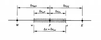
In this figure P is a node and the control volume for P is with length `deltax_(we)`

Now the key step for finite volume method is the integration of governing equation over a control volume to yield a discretized equation as its nodal point P. For the control volume above this gives

Here A - cross sectional area

V - control volume

`barS`=Average value of source over control volume

Now we use the above mentioned interpolation schemes such as upwind, central, QUICK , hybrid and TVD to find the values in the governing equation.

Later will repeat the process at each nodel point all over the domain to obtain at solution for the given equation.

CONCLUSION:

Finally we can say that FVM is really powerful approach to solve the CFD problems . With the help of proper interpolation schemes and accurate use of flux limiters , in case if any discontinuities present we can solve wide range of CFD problems .

Though might be difficult to code and implement in the computers it gives an advantage of its robustness.