Week 9 - FVM Literature Review
Finite Volume Method (FVM):
It derives its name from the fact that in this method the governing PDE is satisfied over a finite-sized control volume. To solve the governing PDE numerically it is first integrated over the finite-sized control volume to get the required discretized equation and the computational domain is split into a set of control volumes known as cells. These control volumes may be of arbitrary shape and size.
Difference between FVM and FDM:
| FVM | FDM |
|
1. The computational domain is divided into discrete numbers of the control volumes. 2. The governing PDE is first integrated over the control volume. 3. The conservation equation is satisfied over each control volume. 4. It can easily be applied to control volume of any arbitrary shape and size. |
1. The computational domain is divided into a discrete numbers of grid points. 2. The governing PDE is discretized over the discrete grid points of the domain. 3. The conservation equation is satisfied over the entire computational domain. 4. It is easy to implement to the grid points which are parallel to cartesian coordinates otherwise grid transformation needs to be done. |
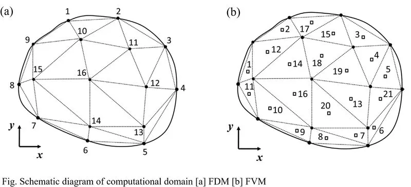
The figure above shows the schematic diagram of the computational domain for both cases.
Need for interpolation scheme:
In FVM the value of the variables are stored at the centre of the cell but in the calculation procedure we need the value of fluxes at the faces of the cell or control volume. So, to calculate the value at the faces of the cell, iinterpolation schemes are required.
The above statement is explained by the following example.
Consider a 1-D heat conduction equation:
`(d)/(dx)[k(dT)/(dx)]=q_g`
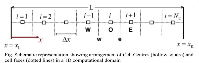
The first step in derivation of the finite volume equation for a given control volume is to integrate the governing equation analytically over the control volume or cell. For the cell i as shown in the figure yields
`int_w^e(d)/(dx)[k(dT)/(dx)]dx=int_w^eq_gdx`
Upon simplification the above can be written as:
`[k(dT)/(dx)]_(e,i)-[k(dT)/(dx)]_(w,i)=Q_(gi)(Deltax)_i`
where the subscript e,i denotes the eastern face of cell i. `(Q_(g))_(i)` denotes the average value of `q_g` over the control volume `Deltax`
Now to calculate the values at faces there is the need of interpolation scheme. Some of the interpolation schemes are:
1. 1st order upwind scheme.
2. Central difference scheme.
3. Quick scheme.
4. Exponential scheme.
Flux Limitter:
Flux limitter are used in high resolution scheme to avoid the spurious oscillation that would otherwise with high order spatial discretization schemes due to shocks, discontinuities or sharp changes in the solution domain. The effect of the flux limitter is to limit the solution gradient near the shock or discontinuities.
Some of the commonly used limiter functions are: CHARM, HCUS, HQUICK, Koren, Osher, etc.