Week 5.1 - Mid term project - Solving the steady and unsteady 2D heat conduction problem

In this challenge, analysis of the 2-D steady and transient heat conduction equation is performed by solving them numerically. The governing equation for the same are as follows:

2-D transient heat conduction equation: `(delT)/(delt)=alpha((del^2T)/(delx^2)+(del^2T)/(dely^2))` where `alpha` is the coefficient of thermal diffusivity.

While in the steady heat conduction equation time derivative is not present: `(del^2T)/(delx^2)+(del^2T)/(dely^2) = 0`.

In the present study, it is assumed that there is neither a heat sink nor a heat source inside the computational domain.

2-D Steady Heat Conduction Equation:

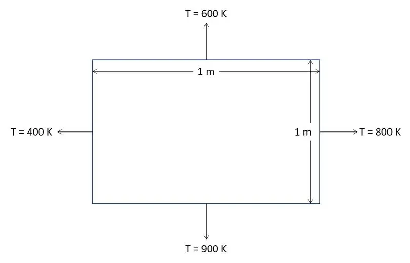
To perform the simulation a square computational domain is considered to have a length of 1 unit. As the governing equation has 2nd order derivative term along both the direction, so to solve it there is need of 4 boundary condition. which is shown in the figure below at all the 4 walls of the domain.

Now, to solve the governing partial differential equation numerically, the 2nd order derivative terms are discretized using the 2nd order accurate central difference scheme. After discretization, the PDE get converted into a linear equation, so after making a proper arrangement the final equation will come like this,

`((2)/(Deltax)^2+(2)/(Deltay^2))T(i,j) = (T(i-1,j)+T(i+1,j))/(Deltax)^2+(T(i,j-1)+T(i,j+1))/(Deltay)^2`. Pictorial representation of grid points are shown below

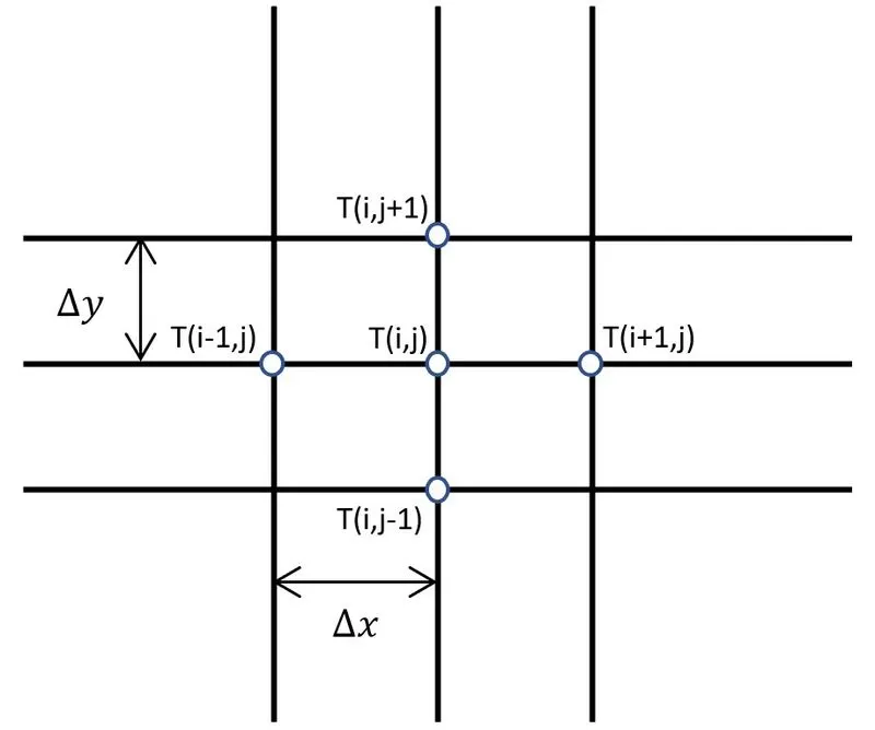
Where all the terms on the Right Hand Side are known as their value are taken from the previous iteration. However, at the very first iteration, the value at grid points inside the computational domain is unknown. So in order to initiate the solution, a random initial guess value is assumed. This initial guess to some extent dictates the number of iteration that requires to converge the solution up to the desired accuracy which means the closer the initial guess to the final solution lesser will be the number of iteration required and vice-versa.

Now there are 3 iterative methods that are being used to solve the above linear equation:

1. Jacobi Method.

2. Gauss-Seidel Method.

3. Successive Over-Relaxation (SOR) Method.

The above equation is solved using the above iterative method in the mentioned computational domain by writing the MATLAB code which is attached below:

% Solving steady 2-D heat conduction equation

clear all
close all
clc

% Defining the parameters
l_x = 1.0;
l_y = 1.0;
nx = 100;                                   % Number of divison along x-direction
ny = nx;                                    % Number of divison along y-direction
x = linspace(0,1,nx+1);
y = linspace(0,1,ny+1);

dx = x(2)-x(1);                             % Grid spacing along x-direction
dy = y(2)-y(1);                             % Grid spacing along x-direction
[X,Y] = meshgrid(x,y);

% Defining boundary condition

T(1:length(x),1:length(y)) = 500;            % This is the initial guess

T(:,1) = 400;                                % Left boundary condition
T(1,:) = 600;                                % Top boundary condition
T(end,:) = 900;                              % Bottom boundary condition
T(:,end) = 800;                              % Right boundary condition

Told = T;

method = 1;                                 % This parameter is used to switch between the solution method
tol = 1e-4;                                 % This defines the tolerance for error
error = 1;                                  % Initialising the error term
iter = 1;                                   % Initialising the iteration variable
r = 1.2;                                    % This is the relaxation factor for SOR method

% This is for Jacobi method.

if method == 1
    while error > tol
        for j = 2:length(y)-1
           for i = 2:length(x)-1
              k = (2/(dx)^2)+(2/(dy)^2);
              term_1 = (Told(i-1,j)+Told(i+1,j))/(dx)^2;
              term_2 = (Told(i,j-1)+Told(i,j+1))/(dy)^2;
              
              T (i,j) = (term_1+term_2)/k;
           end
        end
        error = max(abs(Told(i,j)-T(i,j)));
        Told = T;
        iter = iter + 1;       
    end
 contourf(X,Y,T,10,'ShowText','on')
 xlabel('X-axis')
 ylabel('Y-axis')
 title_text = sprintf('iteration number using Jacobi method = %d', iter);
 title(title_text);
 set(gca,'YDIR','reverse')
end

 % This is for Gauss-Seidel method
 
 if method == 2
    while error > tol
        for j = 2:length(y)-1
           for i = 2:length(x)-1
              k = (2/(dx)^2)+(2/(dy)^2);
              term_1 = (T(i-1,j)+Told(i+1,j))/(dx)^2;
              term_2 = (T(i,j-1)+Told(i,j+1))/(dy)^2;
              
              T (i,j) = (term_1+term_2)/k;
           end
        end
        error = max(abs(Told(i,j)-T(i,j)));
        Told = T;
        iter = iter + 1;       
    end
    contourf(X,Y,T,10,'ShowText','on')
    xlabel('X-axis')
    ylabel('Y-axis')
    title_text = sprintf('iteration number using Gauss-Seidel method = %d', iter);
    title(title_text);
    set(gca,'YDIR','reverse')
 end
 
  % This is for SOR (Successive over-relaxation method) method
  
 if method == 3
    while error > tol
        for j = 2:length(y)-1
           for i = 2:length(x)-1
              k = (2/(dx)^2)+(2/(dy)^2);
              term_1 = (T(i-1,j)+Told(i+1,j))/(dx)^2;
              term_2 = (T(i,j-1)+Told(i,j+1))/(dy)^2;
              
              T (i,j) = ((1-r)*Told(i,j))+ (r*(term_1+term_2)/k);   % T_gauss_seidel is used
           end
        end
        error = max(abs(Told(i,j)-T(i,j)));
        Told = T;
        iter = iter + 1;       
    end
    contourf(X,Y,T,10,'ShowText','on')
    xlabel('X-axis')
    ylabel('Y-axis')
    title_text = sprintf('iteration number using SOR method = %d', iter);
    title(title_text);
    set(gca,'YDIR','reverse')
 end
 

In the code following parameter is considered:

Initial guess at all the internal grid points is taken as `T = 500 K`. The number of divisions along the x and y-direction are taken equal, `nx = ny = 100.` which means grid spacing along both the direction is equal. The tolerance for the error is taken as `10^(-4)`

Error is defined as the maximum of the absolute value of the difference of the temperature of consecutive iteration at all the grid points inside the computational domain.

1. Using the Jacobi method:

The plot obtained using the Jacobi method is attached below:

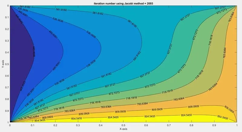
So, to attain the desired tolerance level for the error Jacobi method took 2093 iterations. However, this iteration value will change as one changes the initial condition, boundary condition as well as grid spacing.

2. Using the Gauss-Seidel method:

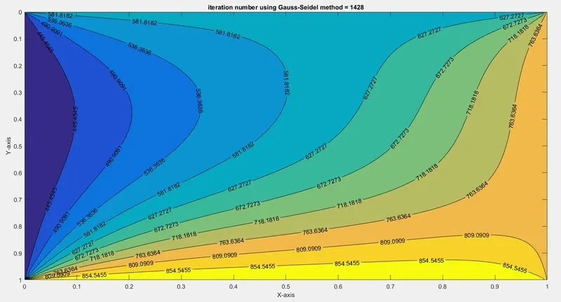
The Gauss-Seidel method is slightly different from the Jacobi iterative method. In the Jacobi method in an iteration, the value of the previous iteration is used while in the Gauss-Seidel method the values keep on updating inside an iteration. The advantage of this procedure is that solution gets converged at a faster rate, as a result, the number of iteration required is less. The same is observed in the present study. While using the Gauss-Seidel method number of iteration required is 1428 which is less than the Jacobi method.

3. Using the Successive Over-Relaxation (SOR) method:

This is the improved version of the Jacobi method or Gauss-Seidel method. In this, a parameter (say r) is introduced which enhances or increases the rate of convergence of the iterative method. Mathematically,

`T(i,j) = (1-r)*T_(old)(i,j) + r(T_(GS) or T_(Jacobi))` where GS stands for Gauss-Seidel and r is known as the relaxation factor.

If `r > 1`, over-relaxed factor

If `r < 1`, under-relaxed factor

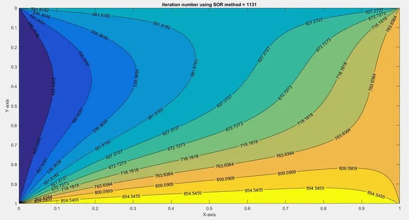
However, there is not any thumb rule to choose the value for this parameter. Care must be taken while solving the equation using this method because the relaxation factor helps to increase the convergence rate but beyond some values, it slows down the convergence rate or gives the wrong result. So, the result obtained from this method must be validated from the existing result or with the result obtained from other methods.

In the present plot obtained, a relaxation factor, r = 1.2 is taken and the iteration required is 1131 which is less than Gauss-Seidel as well as the Jacobi method.

Conclusion:

1. The rate of convergence of the solution is higher for the SOR method followed by the Gauss-Seidel method and least for the Jacobi method. However, the rate of convergence of the SOR method depends upon the relaxation factor r, whose value is decided based on the hit and trial method. In the present analysis, it is found that for `r< 1` the rate of convergence decreases, and for `r>2` it results in an erroneous solution.

2. The variation of temperature contour is smooth in the entire domain which is because of the fact that the governing equation is elliptic in nature.

2-D Unsteady Heat Conduction Analysis:

Now coming to the 2-D unsteady heat conduction analysis, the governing equation is: `(delT)/(delt)=alpha((del^2T)/(delx^2)+(del^2T)/(dely^2))` where `alpha` is the coefficient of thermal diffusivity.

So, to solve the above PDE there are 3 methods:

1. Explicit Formulation.

2. Implicit Formulation

1. Jacobi method.
2. Gauss-Seidel method.
3. Successive Over-Relaxation method.

3. Crank-Nicolson method.

In the present study, two methods have been covered explicit formulation and implicit formulation.

Explicit formulation:

Discretizing the above governing equation using 2nd order accurate central-difference scheme to spatial derivative and 1st order accurate temporal derivative and writing them in explicit formulation we will get

`T_(i,j)^(n+1) = (1-(2alphaDeltat)/(Deltax)^2-(2alphaDeltat)/(Deltay)^2)*T_(i,j)^n+(alphaDeltat)/(Deltax)^2(T_(i-1,j)^n+T_(i+1,j)^n)+(alphaDeltat)/(Deltay)^2(T_(i,j-1)^n+T_(i,j+1)^n)`, So in this equation everything is known on the RHS and only one unknown is there. So it is easy to solve this equation. The only issue with this formulation is that for a stable solution the coefficient associated with all variables should be positive which implies

`(1-(2alphaDeltat)/(Deltax)^2-(2alphaDeltat)/(Deltay)^2)>=0`

`=> (alphaDeltat)/(Deltax)^2+(alphaDeltat)/(Deltay)^2<=1/2`, if `Delta x =Delta y` (which is assumed in the present case)

`=> (alpha Deltat)/(Deltax)^2<=1/4`

`=> Delta t = (Deltax)^2/(4alpha)`. So this is the restriction on the time steps that can be used to get a stable solution for a given grid spacing and thermal diffusion coefficient and the same formula is being used inside the MATLAB code to automatically calculate the time step as the grid spacing and the thermal diffusion coefficient is changed.

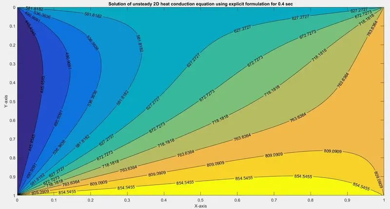
As this is a transient problem, so we need an initial condition also to solve the problem. The problem is simulated for a period of 0.4 sec.

The obtained temperature field is attached below:

The code for the explicit formulation is attached below:

% Solving unsteady 2-D heat conduction equation using explicit formulation

clear all
close all
clc

% Defining the parameters
l_x = 1.0;
l_y = 1.0;
nx = 100;
ny = nx;
x = linspace(0,1,nx+1);
y = linspace(0,1,ny+1);

alpha = 1.5;                                % This is coefficient of diffusivity

dx = x(2)-x(1);                             % Grid spacing along x-direction
dy = y(2)-y(1);                             % Grid spacing along y-direction
[X,Y] = meshgrid(x,y);

dt = ((dx)^2)/(4*alpha);                    % Time step following the stability condition
nt = 0.4/dt;                                % Number of time step = simulation time / time step

% Defining boundary condition and initial condition

T(1:length(x),1:length(y)) = 600;           % This is the initial condition

T(:,1) = 400;                               % Left boundary condition
T(1,:) = 600;                               % Top boundary condition
T(end,:) = 900;                             % Bottom boundary condition
T(:,end) = 800;                             % Right boundary condition

Told = T;
ct = 1;

for k = 1:nt                                % This loop is for varitaion over time.
   % Loop for spatial variation
   for j = 2:length(y)-1
      for i = 2:length(x)-1
         k_1 = (alpha*dt)/((dx)^2);
         k_2 = (alpha*dt)/((dy)^2);
         
         term_1 = (1-(2*k_1)-(2*k_2))*(Told(i,j));
         term_2 = k_1*(Told(i-1,j)+Told(i+1,j));
         term_3 = k_2*(Told(i,j-1)+Told(i,j+1));
         
         T(i,j) = term_1+term_2+term_3;
      end
   end
    Told = T;
    contourf(X,Y,T,10,'ShowText','on')
    xlabel('X-axis')
    ylabel('Y-axis')
    title('Solution of unsteady 2D heat conduction equation using explicit formulation for 0.4 sec')
    set(gca,'YDIR','reverse')
    pause(0.00003)
    
    q(ct) = getframe(gcf);
    ct = ct +1;
end

% To create animation movie
movie(q)
videofile = VideoWriter('Explicit_Heat_Conduction.avi', 'uncompressed avi'); % VideoWriter is a command and is case-sensitive
open(videofile)
writeVideo(videofile,q)
close(videofile)

Implicit Formulation:

Now coming to another formulation to solve the transient equation numerically. After discretizing the governing PDE we will get the following:

`(1+(2alphaDeltat)/(Deltax)^2+(2alphaDeltat)/(Deltay)^2)*T_(i,j)^(n+1) = T_(i,j)^n +(alphaDeltat)/(Deltax)^2``(T_(i-1,j)^(n+1) + T_(i+1,j)^(n+1) )+ (alphaDeltat)/(Deltay)^2(T_(i,j-1)^(n+1) + T_(i,j+1)^(n+1) )`

From above equation one can find that there is only one known value `(T_(i,j)^n)`and rest of the variable is still unknown. So to solve the above equation we have to follow iterative method like the Jacobi method, the Gauss-Seidel method or SOR method.

Before jumping into any method it is necessary to understand how this iterative method is going to work. For the same a flow diagram is attached below:

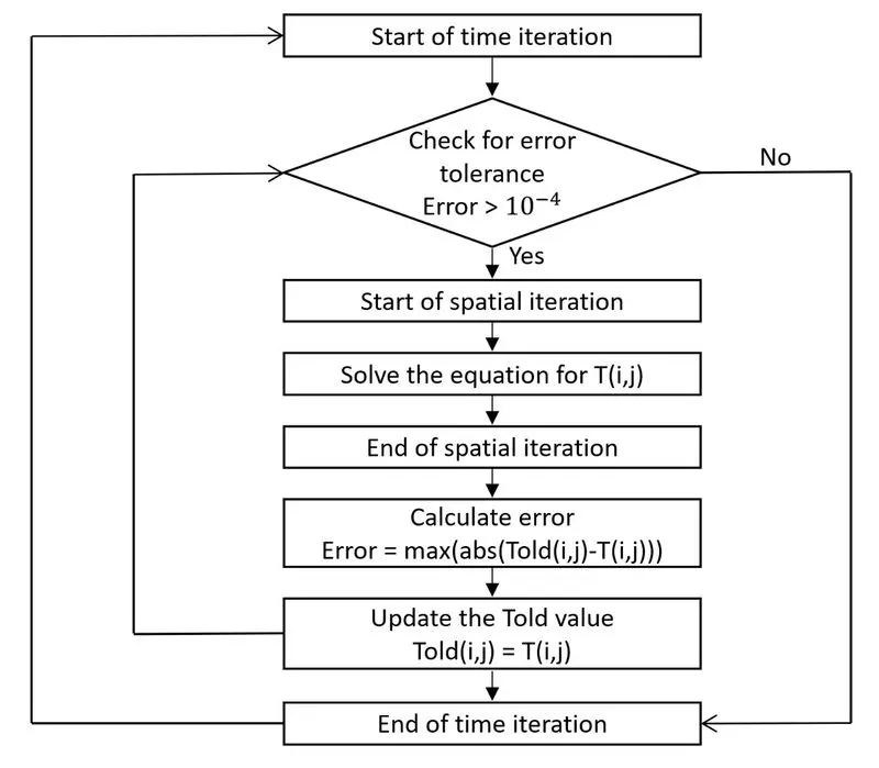
where `T_(old)`is the value taken from the previous iteration. (NOTE: Don't get confused the previous iteration with the previous time iteration. Both are different.) Within a time iteration, several iterations take place inside the computational domain and continue until the tolerance for the error is satisfied.

MATLAB code for the numerical solution of 2-D unsteady heat conduction equation using implicit formulation is attached below:

% Solving unsteady 2-D heat conduction equation using implicit formulation

clear all
close all
clc

% Defining the parameters
l_x = 1.0;
l_y = 1.0;
nx = 100;
ny = nx;
x = linspace(0,1,nx+1);
y = linspace(0,1,ny+1);

alpha = 1.5;

dt = 0.01;
nt = 40;

dx = x(2)-x(1);
dy = y(2)-y(1);
[X,Y] = meshgrid(x,y);

% Defining boundary condition

T(1:length(x),1:length(y)) = 500;            % This is the initial guess

T(:,1) = 400;                                % Left boundary condition
T(1,:) = 600;                                % Top boundary condition
T(end,:) = 900;                              % Bottom boundary condition
T(:,end) = 800;                              % Right boundary condition

Told = T;                                   % This value is from previous iteration
T_prev_time = T;                            % This value is from previous time iteration
T_GS = ones(length(x),length(y));

method = 3;                                 % This parameter is used to switch between the solution method
tol = 1e-4;                                 % This defines the tolerance for error
error = 1;                                  % Initialising the error term
iter = 0;                                   % Initialising the iteration variable
r = 1.3;                                    % This is the relaxation factor for SOR method

% For Jacobi method

if method == 1;
   for k = 1:nt
       error = 1.0;
       while error > tol
          for j = 2:length(y)-1
             for i = 2:length(x)-1
                 k_1 = (alpha*dt)/((dx)^2);
                 k_2 = (alpha*dt)/((dy)^2);
                 
                 term_1 = k_1*(Told(i-1,j)+Told(i+1,j));
                 term_2 = k_2*(Told(i,j-1)+Told(i,j+1));
                 
                 T(i,j) = (T_prev_time(i,j) + term_1 + term_2)/(1+(2*k_1)+(2*k_2));
             end
          end
          error = max(abs(Told(i,j)-T(i,j)));
          Told = T;
          iter = iter+1;
       end
        %Told = T;
        T_prev_time = T;
        contourf(X,Y,T,10,'ShowText','on')
        xlabel('X-axis')
        ylabel('Y-axis')
        title('2D Unsteady Heat Conduction Equation')
        title_text = sprintf('2D Unsteady Heat Conduction Equation (Iteration number using Jacobi method = %d)', iter);
        title(title_text);
        set(gca,'YDIR','reverse')
        pause(0.002)
   end
end

% This is for Gauss-Seidel Method

if method == 2;
   for k = 1:nt
       error = 1.0;
       while error > tol
          for j = 2:length(y)-1
             for i = 2:length(x)-1
                 k_1 = (alpha*dt)/((dx)^2);
                 k_2 = (alpha*dt)/((dy)^2);
                 
                 term_1 = k_1*(T(i-1,j)+Told(i+1,j));
                 term_2 = k_2*(T(i,j-1)+Told(i,j+1));
                 
                 T(i,j) = (T_prev_time(i,j) + term_1 + term_2)/(1+(2*k_1)+(2*k_2));
             end
          end
          error = max(abs(Told(i,j)-T(i,j)));
          Told = T;
          iter = iter+1;
       end
        %Told = T;
        T_prev_time = T;
        contourf(X,Y,T,10,'ShowText','on')
        xlabel('X-axis')
        ylabel('Y-axis')
        %iter = iter+1;
        title_text = sprintf('2D Unsteady Heat Conduction Equation (Iteration number using Gauss-Seidel method = %d)', iter);
        title(title_text);
        set(gca,'YDIR','reverse')
        pause(0.002)
   end
end

% This is for Successive Over Relaxation method

if method == 3;
   for k = 1:nt
       error = 1.0;
       while error > tol
          for j = 2:length(y)-1
             for i = 2:length(x)-1
                 k_1 = (alpha*dt)/((dx)^2);
                 k_2 = (alpha*dt)/((dy)^2);
                 
                 term_1 = k_1*(T(i-1,j)+Told(i+1,j));
                 term_2 = k_2*(T(i,j-1)+Told(i,j+1));
                 
                 T_GS(i,j) = (T_prev_time(i,j) + term_1 + term_2)/(1+(2*k_1)+(2*k_2));
                 
                 T(i,j) = (1-r)*Told(i,j) + r*T_GS(i,j);
             end
          end
          error = max(abs(Told(i,j)-T(i,j)));
          Told = T;
          iter = iter+1;
       end
        %Told = T;
        T_prev_time = T;
        contourf(X,Y,T,10,'ShowText','on')
        xlabel('X-axis')
        ylabel('Y-axis')
        %iter = iter+1;
        title_text = sprintf('2D Unsteady Heat Conduction Equation (Iteration number using SOR method = %d)', iter);
        title(title_text);
        set(gca,'YDIR','reverse')
        pause(0.002)
   end
end

1. The Jacobi method:

So mathematically `T_(i,j)^(n+1)` can be written as

`(1+(2alphaDeltat)/(Deltax)^2+(2alphaDeltat)/(Deltay)^2)*T_(i,j)^(n+1) = T_(i,j)^n +(alphaDeltat)/(Deltax)^2``(Told_(i-1,j)^(n+1) + Told_(i+1,j)^(n+1) )+ (alphaDeltat)/(Deltay)^2(Told_(i,j-1)^(n+1) + Told_(i,j+1)^(n+1) )`

The result obtained is attached below:

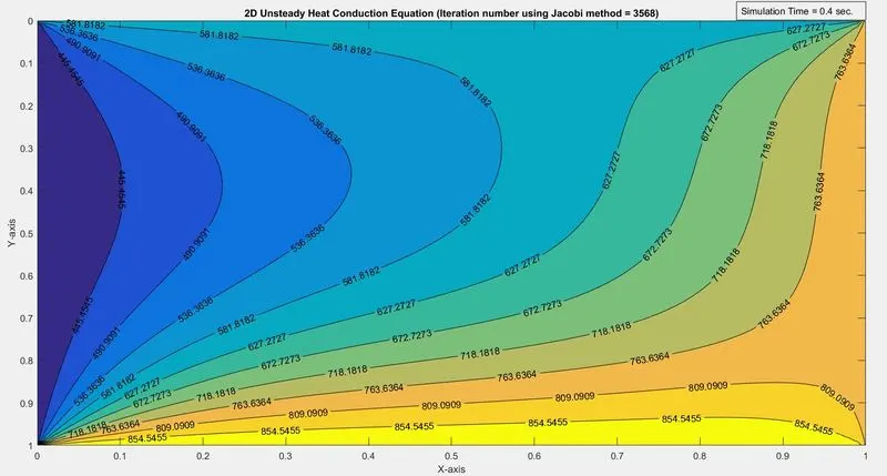
The number of iteration required is 3568.

2. The Gauss Seidel method:

Gauss-Seidel method is an improved version of the Jacobi method. In this, the updated values are considered within an iteration itself. Due to this, the rate of convergence is higher for this method as compared to the Jacobi method. The result obtained using the Gauss-Seidel method is attached below:

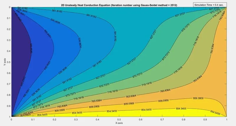
The number of iteration required is 2512 which is lower than that of the Jacobi method.

3. Successive Over-Relaxation method:

Mathematically,

`T_(i,j)^(n+1) = (1-r)*(T_(old))_(i,j)^(n+1) + r*(T_(GS)or T_(Jacobi))`

This is the enhanced version of the Gauss-Seidel method or the Jacobi method. This is because of the relaxation parameter, r.

If `r > 1`, over-relaxed factor

If `r < 1`, under-relaxed factor.

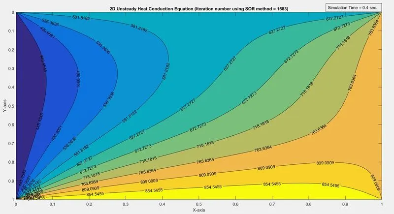
In the present result obtained the value of r is taken as 1.3 and the number of iteration required is 1583 which is the least among the three mentioned iterative methods used.

Conclusion (Transient Analysis):

1. Explicit formulation is easier to code but there is a restriction on the time steps, `Deltat prop (1)/(Deltax)^2`, so as we reduce the grid spacing, the time step has to be reduced thus increases the computational time.

2. In implicit formulation number of unknowns are higher which can be solved by either direct method (requires large computational storage) or iterative method. In the present study, iterative methods are used.

3. Implicit formulation does not have any restriction on the time step so a large time step can be used but as one tries to increase the time step then the truncation error will increase.