Week 11 - Simulation of Flow through a pipe in OpenFoam
Laminar flow through a circular pipe:
In this challenge, the flow physics for the laminar flow through a circular pipe is being studied using OpenFOAM. So to begin with the first thing is to create the geometry using the blockMeshDict script file. As the laminar flow through the circular pipe is an axisymmetric flow so instead of creating the entire pipe only a wedge section is being considered for the study. Below a schematic diagram of the wedge section is attached.
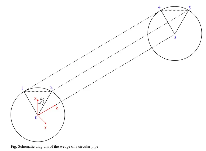
To automate the blockMeshDict script file help of file parsing is being used. Actually, the code is written in MATLAB where it takes the input as the radius, length, wedge angle and upon execution, it generates the blockMeshDict file.
The MATLAB code is attached below:
clear all
close all
clc
% For calculation of length
% Entry length = 0.05*Re*D
Re = 2100;                      % Reynolds number of the flow
r = 12.5;                       % radius of tube in mm

Le = 0.05*Re*(2*r);             % Entry length

l = Le+0.2*Le;                  % length of tube in mm
theta = (pi/45);                % Wedge angle
nx = 20;                        % Along radial direction
ny = 1;                         % Along the wedge faces
nz = 1000;                      % Along the longitudinal axis

f1 =fopen('blockMeshDict.txt','w');

fprintf(f1,'FoamFile\n');
fprintf(f1,'{\nversion 2.0;\n');
fprintf(f1,'format ascii;\n');
fprintf(f1,'class dictionary;\n');
fprintf(f1,'object blockMeshDict;\n}\n');
fprintf(f1,'convertToMeters 1e-3;\n\n');

fprintf(f1,'vertices\n');
fprintf(f1,'(\n');
fprintf(f1,'(%f %f %f)\n', 0, 0, 0);
fprintf(f1,'(%f %f %f)\n', r*cos(theta/2), -r*sin(theta/2), 0);
fprintf(f1,'(%f %f %f)\n\n', r*cos(theta/2), r*sin(theta/2), 0);

fprintf(f1,'(%f %f %f)\n', 0, 0, l);
fprintf(f1,'(%f %f %f)\n', r*cos(theta/2), -r*sin(theta/2), l);
fprintf(f1,'(%f %f %f)\n', r*cos(theta/2), r*sin(theta/2), l);

fprintf(f1,');\n\n');

fprintf(f1,'blocks\n');
fprintf(f1,'(\n');
fprintf(f1,'hex (0 1 2 0 3 4 5 3)');
fprintf(f1,' (%6.0f %6.0f %6.0f)', nx,ny,nz);
fprintf(f1,' simpleGrading (0.2 1 1)\n');
fprintf(f1,');\n\n');

fprintf(f1,'edges\n');
fprintf(f1,'(\n');
fprintf(f1,'arc 1 2');
fprintf(f1,' (%f %f %f)\n', r, 0, 0);
fprintf(f1,'arc 4 5');
fprintf(f1,' (%f %f %f)\n', r, 0, l);
fprintf(f1,');\n\n');

fprintf(f1,'boundary\n\n');

fprintf(f1,'(\n');
fprintf(f1,'topWall\n');
fprintf(f1,'{\n');
fprintf(f1,'type wall;\n');
fprintf(f1,'faces\n');
fprintf(f1,'(\n');
fprintf(f1,'(1 2 5 4)\n');
fprintf(f1,');\n');
fprintf(f1,'}\n\n');

fprintf(f1,'inlet\n');
fprintf(f1,'{\n');
fprintf(f1,'type patch;\n');
fprintf(f1,'faces\n');
fprintf(f1,'(\n');
fprintf(f1,'(0 2 1 0)\n');
fprintf(f1,');\n');
fprintf(f1,'}\n\n');

fprintf(f1,'outlet\n');
fprintf(f1,'{\n');
fprintf(f1,'type patch;\n');
fprintf(f1,'faces\n');
fprintf(f1,'(\n');
fprintf(f1,'(3 4 5 3)\n');
fprintf(f1,');\n');
fprintf(f1,'}\n\n');

fprintf(f1,'bottom\n');
fprintf(f1,'{\n');
fprintf(f1,'type empty;\n');
fprintf(f1,'faces\n');
fprintf(f1,'(\n');
fprintf(f1,'(0 3 3 0)\n');
fprintf(f1,');\n');
fprintf(f1,'}\n\n');

fprintf(f1,'front\n');
fprintf(f1,'{\n');
fprintf(f1,'type wedge;\n');
fprintf(f1,'faces\n');
fprintf(f1,'(\n');
fprintf(f1,'(0 3 5 2)\n');
fprintf(f1,');\n');
fprintf(f1,'}\n\n');

fprintf(f1,'back\n');
fprintf(f1,'{\n');
fprintf(f1,'type wedge;\n');
fprintf(f1,'faces\n');
fprintf(f1,'(\n');
fprintf(f1,'(0 3 4 1)\n');
fprintf(f1,');\n');
fprintf(f1,'}\n\n');

fprintf(f1,');\n\n');

fprintf(f1,'mergePatchPairs\n');
fprintf(f1,'(\n');
fprintf(f1,');');

fclose(f1);
The parameters are considered as follows: Reynolds number, Re = 2100,
The diameter of the tube is assumed as, D = 25 mm,
For water, density `rho = 1.2567(kg)/m^3`
Dynamic viscosity, `mu=1.86xx10^-5Pa.s`, based upon the above parameters the following values are being calculated:
`V_(i nl et)=(Rexxmu)/(rhoxxD)=1.2432m/s`
At the inlet pressure gradient is set as zero, for the wall of the tube no-slip boundary condition is used and pressure gradient is set to zero, at the outlet gauge pressure is zero and the velocity gradient is set as zero and at the two walls of the wedge, the boundary condition is used.
The wedge angle for the present study is kept as `4^o`.
Upon simulating the above flow following results are obtained:
1. Velocity profile of fully developed flow:
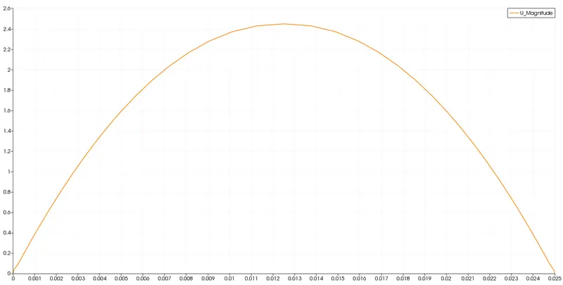
So the obtained velocity profile is parabolic in nature and the value of `V_max=2.4 m/s` (approximately).
While theoretically `V_max=2xxV_(i nl et)=2.4864m/s` which is quite close.
2. Entry length:
It is defined as the length measured from the inlet to the point beyond which the velocity gradient along the flow direction becomes zero. This also gives the indication of the fully developed flow.
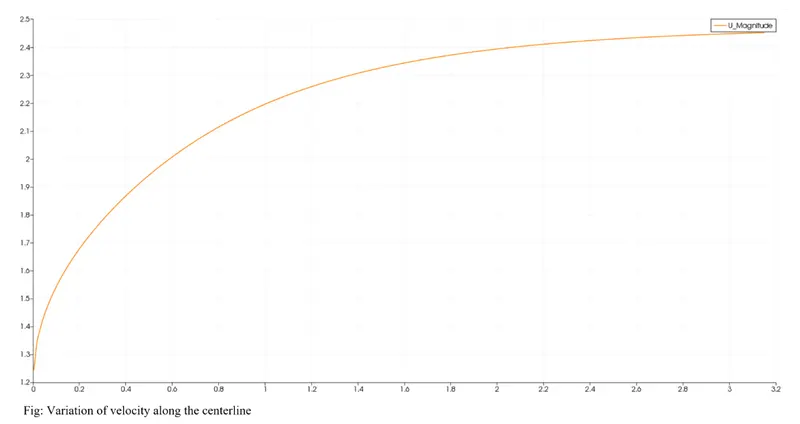
From the plot, it can be seen that the entry length is 2.8 m approximately. While using the empirical relation,
`L_e=0.05xxRexxD=2.625 m`
3. Wall shear stress:
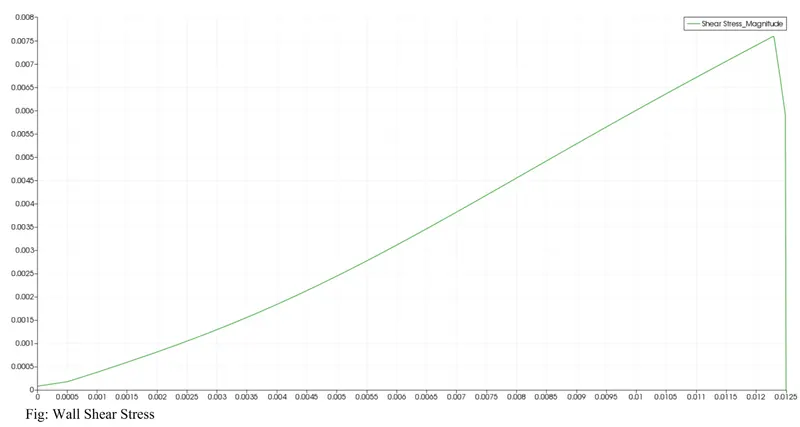
At the wall, the value of shear stress is maximum and is equal to `0.0075N/m^2`
Analytically, `tau_w=(4muxxV_(avg))/R=0.00739N/m^2`
4. Pressure Loss:
Analytically the pressure (Kinematic) drop is given as,
`(DeltaP)/(rho)=(32nuLV_(avg))/D^2=2.9674m^2/s^2`
While the plot obtained from the simulation is attached below.
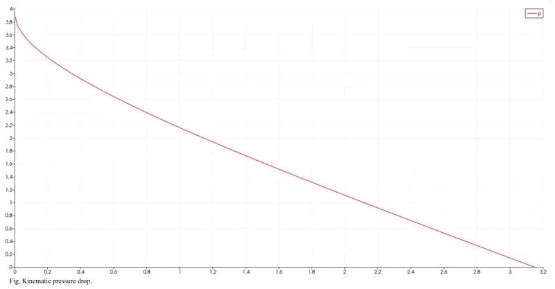
The pressure (kinematic) drop from the plot is approximately `3.85 m^2/s^2`.
Conclusion:
The result obtained from the simulation is compared with the analytically calculated results. It is being observed that numerically obtained results are very much close to the analytically obtained result.
Thus, the numerical simulation is consistent with the actual flow physics.