Week 12 - Validation studies of Symmetry BC vs Wedge BC in OpenFOAM vs Analytical H.P equation

Validation Study of symmetry BC and wedge BC:

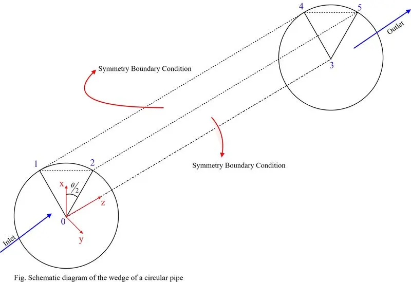
In this study, the simulation result obtained from both boundary conditions is compared for the laminar flow through a pipe. In this present study, the simulation is performed by implementing the symmetry boundary condition to the two faces as shown in the figure below.

Analytical Calculation:

Reynolds number, Re = 2100; Diameter, D = 25 mm; the simulation is performed for air so, dynamic viscosity, `mu= 1.86xx10^-5 Pa*s`

Density, `rho=1.2567 m^3/s`

Therefore, Inlet velocity, `V_(i nl et)=(Rexxmu)/(rhoxxD)=1.2432 m/s` (`V_(avg)=V_(i nl et)`)

`V_(max)=2xxV_(i nl et)=2.4864 m/s`

Hydrodynamic entry length, `L_e=0.05xxRexxD=2.625m`

Therefore, Length of the pipe is taken as, `L = 1.2L_e=3.15 m`

Kinematic Pressure loss, `(Delta P)/(rho)=(32nuLV_(avg))/(D^2)=2.9674(m^2)/s^2`

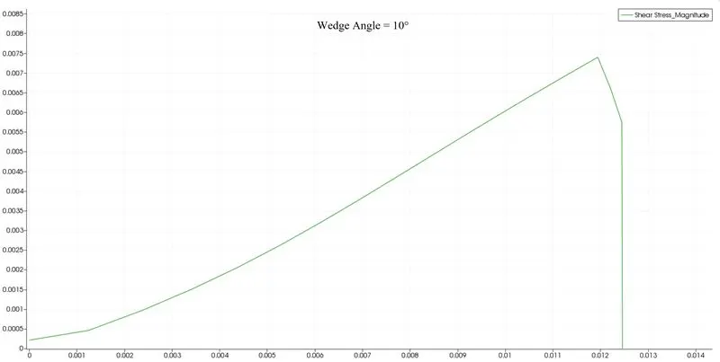
Wall shear stress, `tau_(w)=(8muV_(avg))/D=0.007397N/m^2`

Now to perform the simulation blockMeshDict script file is to be generated first. This blockMeshDict is generated by using the file parsing method. Below the MATLAB code for the same is being attached:

clear all
close all
clc
% For calculation of length
% Entry length = 0.05*Re*D
Re = 2100;                      % Reynolds number of the flow
r = 12.5;                       % radius of tube in mm

Le = 0.05*Re*(2*r);             % Entry length

l = Le+0.2*Le;                  % length of tube in mm
theta = (pi/4);                % Wedge angle
nx = 20;                        % Along radial direction
ny = 1;                         % Along the wedge faces
nz = 1000;                      % Along the longitudinal axis

f1 =fopen('blockMeshDict.txt','w');

% fprintf(f1,'FoamFile\n');
% fprintf(f1,'{\nversion 2.0;\n');
% fprintf(f1,'format ascii;\n');
% fprintf(f1,'class dictionary;\n');
% fprintf(f1,'object blockMeshDict;\n}\n');
% fprintf(f1,'convertToMeters 1e-3;\n\n');

fprintf(f1,'vertices\n');
fprintf(f1,'(\n');
fprintf(f1,'(%f %f %f)\n', 0, 0, 0);
fprintf(f1,'(%f %f %f)\n', r*cos(theta/2), -r*sin(theta/2), 0);
fprintf(f1,'(%f %f %f)\n\n', r*cos(theta/2), r*sin(theta/2), 0);

fprintf(f1,'(%f %f %f)\n', 0, 0, l);
fprintf(f1,'(%f %f %f)\n', r*cos(theta/2), -r*sin(theta/2), l);
fprintf(f1,'(%f %f %f)\n', r*cos(theta/2), r*sin(theta/2), l);

fprintf(f1,');\n\n');

fprintf(f1,'blocks\n');
fprintf(f1,'(\n');
fprintf(f1,'hex (0 1 2 0 3 4 5 3)');
fprintf(f1,' (%6.0f %6.0f %6.0f)', nx,ny,nz);
fprintf(f1,' simpleGrading (0.2 1 1)\n');
fprintf(f1,');\n\n');

fprintf(f1,'edges\n');
fprintf(f1,'(\n');
fprintf(f1,'arc 1 2');
fprintf(f1,' (%f %f %f)\n', r, 0, 0);
fprintf(f1,'arc 4 5');
fprintf(f1,' (%f %f %f)\n', r, 0, l);
fprintf(f1,');\n\n');

fprintf(f1,'boundary\n\n');

fprintf(f1,'(\n');
fprintf(f1,'topWall\n');
fprintf(f1,'{\n');
fprintf(f1,'type wall;\n');
fprintf(f1,'faces\n');
fprintf(f1,'(\n');
fprintf(f1,'(1 2 5 4)\n');
fprintf(f1,');\n');
fprintf(f1,'}\n\n');

fprintf(f1,'inlet\n');
fprintf(f1,'{\n');
fprintf(f1,'type patch;\n');
fprintf(f1,'faces\n');
fprintf(f1,'(\n');
fprintf(f1,'(0 2 1 0)\n');
fprintf(f1,');\n');
fprintf(f1,'}\n\n');

fprintf(f1,'outlet\n');
fprintf(f1,'{\n');
fprintf(f1,'type patch;\n');
fprintf(f1,'faces\n');
fprintf(f1,'(\n');
fprintf(f1,'(3 4 5 3)\n');
fprintf(f1,');\n');
fprintf(f1,'}\n\n');

fprintf(f1,'bottom\n');
fprintf(f1,'{\n');
fprintf(f1,'type empty;\n');
fprintf(f1,'faces\n');
fprintf(f1,'(\n');
fprintf(f1,'(0 3 3 0)\n');
fprintf(f1,');\n');
fprintf(f1,'}\n\n');

fprintf(f1,'front\n');
fprintf(f1,'{\n');
fprintf(f1,'type symmetry;\n');
fprintf(f1,'faces\n');
fprintf(f1,'(\n');
fprintf(f1,'(0 3 5 2)\n');
fprintf(f1,');\n');
fprintf(f1,'}\n\n');

fprintf(f1,'back\n');
fprintf(f1,'{\n');
fprintf(f1,'type symmetry;\n');
fprintf(f1,'faces\n');
fprintf(f1,'(\n');
fprintf(f1,'(0 3 4 1)\n');
fprintf(f1,');\n');
fprintf(f1,'}\n\n');

fprintf(f1,');\n\n');

fprintf(f1,'mergePatchPairs\n');
fprintf(f1,'(\n');
fprintf(f1,');');

fclose(f1);

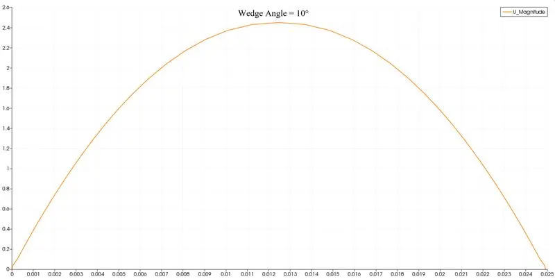
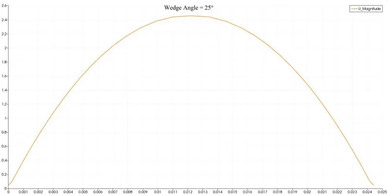
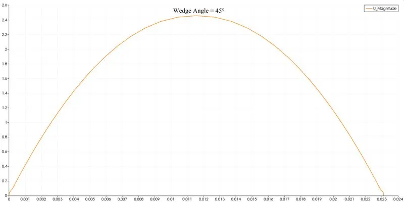
Below the plots for various wedge angles is being attached.

1. Velocity profile of fully developed flow:

2. Kinematic Pressure Loss:

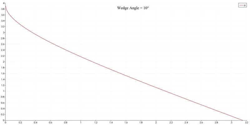
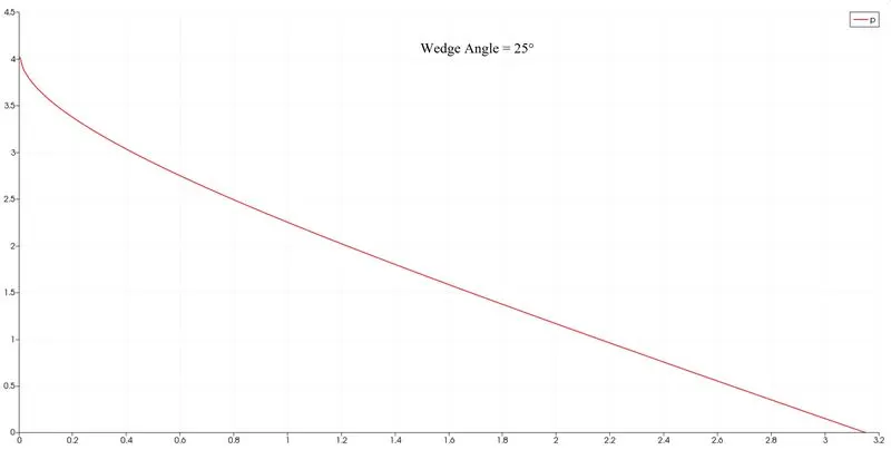
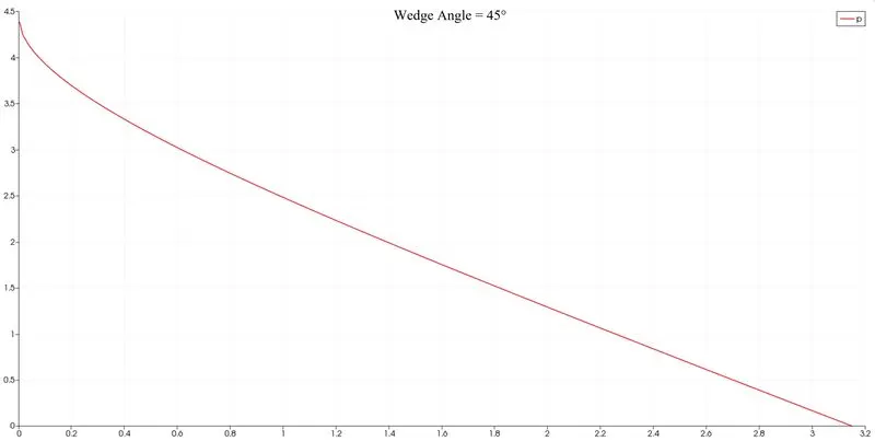
3. Wall Shear Stress:

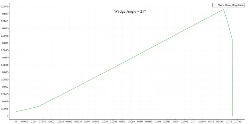
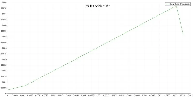
4. Entry Length:

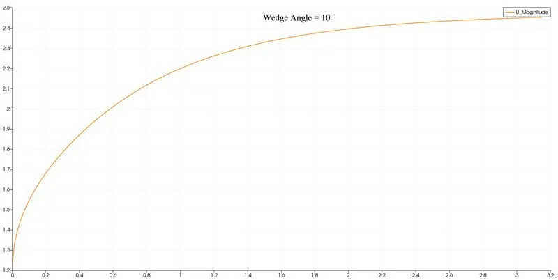
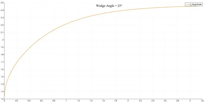
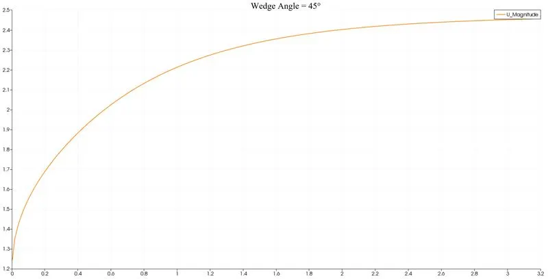
Comparison among the values are presented in the table below:

	`(Delta P)/rho(m^2/s^2)`	`V_(max) (m/s)`	`tau_w(N/m^2)`	`L_e(m)`
Analytical	2.9674	2.4864	0.007397	2.625
Wedge BC (`theta = 4^@`)	3.85	2.4	0.0075	2.8
Symmetry BC (`theta = 10^@`)	3.9	2.45	0.0074	2.8
Symmetry BC (`theta = 25^@`)	4.0	2.454	0.00726	2.85
Symmetry BC (`theta = 45^@`)	4.4	2.45	0.00767	2.9

Conclusion:

1. The result obtained using the wedge BC is closer to the analytical result as compared to the symmetry BC.

2. In symmetry BC small wedge angle gives a good result and as the wedge angle is increased the error in the solution increases.