Week 7 - Simulation of a 1D Super-sonic nozzle flow simulation using Macormack Method
Simulation of Quasi-1D flow in convergent-divergent nozzle:
When the variation of cross-section area is gradual, it is convenient and sufficiently accurate to neglect the variation of flow properties along the y and z-direction and to assume the flow properties to be a function of x only, such a flow is known as quasi-1D flow. With this assumption, the governing equations are modified and solved numerically using the MacCormack method.
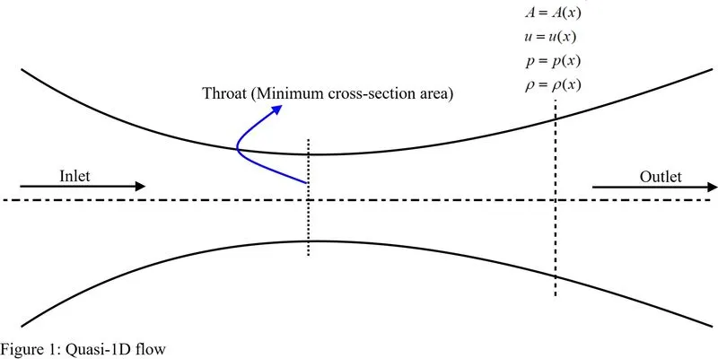
To solve the governing equations numerically one can have two forms:
1. Non-conservative governing equations
2. Conservative governing equations
Mathematically both the form of governing equations are the same. Only they differ from each other numerically and the approach of solving them and definitely there is a slight difference in the result obtained from them which is being covered in this study through this problem.
Non-Conservative governing equation:
Following are the governing equation in the non-conservative form:
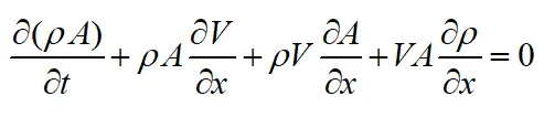
Continuity equation:
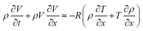
Momentum equation:
Energy equation:
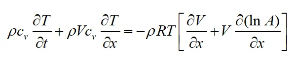
where,

These equations are in dimensional form. But for the ease of convenience of comparison with the analytical solution the above set of equations are non-dimensionalized using the following variables.
Dimensionless density = `(rho)/(rho_0)`, where `rho_0` is the stagnation density or the reservoir density
Dimensionless Temperature = `(T)/T_0`, where `T_0` is the stagnation temperature,
Dimensionless velocity = `(V)/a_0`, where `a_o`is the velocity of sound at the stagnation temperature
Dimensionless length = `(x)/L`, where L is the length of the nozzle
Dimensionless area = `(A)/A^(**)`, `A^(**)` is the area of the throat
Dimensionless time = `t/(L//a_0)`
So finally the non-dimensionalized governing equation is as follows:
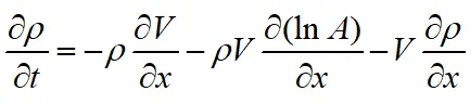
Continuity equation:
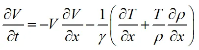
Momentum equation:
Energy equation:

To solve the above set of equations numerically MacCormack method is used. It is a two-step method to calculate the time derivative term.
1st Step: Predictor step
In this step, the time derivative term is being calculated by discretizing all the spatial derivative terms using the 1st order forward difference scheme. After calculating the time derivative, the value of the primitive variables i.e. `rho, V, and T` is updated which is being used in the next step.
2nd step: Corrector step
In the step again time derivative is being calculated using the updated value of primitive variables but this time the spatial derivative is calculated using the 1st order backward difference scheme. So, once this step is done then the average of the time derivative calculated in both the step is calculated to get the final time derivative. After this final update of the primitive variable is done and this process is iterated in every time step.
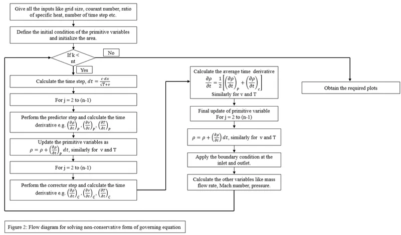
Below is the flow diagram for solution procedure of non-conservative form of governing equation
Courant Number:
As the governing set of equations is hyperbolic with respect to time. So the time step should be kept such that it will give a stable solution. From the stability analysis, it is being found that the time step can be determined using the following relation
`Deltat = (c*dx)/(a+v)`, where c is the courant number, a is the local speed of sound, v is the local flow velocity. When written in non-dimensionalized form `Deltat` is given by
`(Delta t)=(c*dx)/(sqrt(T)+v)`. Generally, for a linear hyperbolic equation, the stability criteria suggest that the value of the courant number should be less than 1. As the present set of governing equations is non-linear in nature so this value of the courant number gives good guidance to consider the value of the courant number for this case. So, in this study by varying the CFL number steady-state solution is being obtained which is listed in the table below.
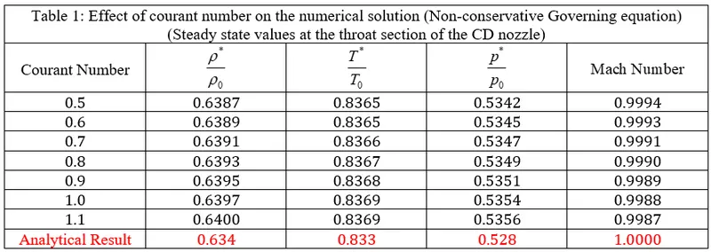
So, it can be concluded from the above table that for the CFL number equal to 0.5, the numerical solution is closer to the analytical solution and as the CFL number is increased there is a marginal departure from the exact solution. Also, it can be observed that a stable solution is being obtained for CFL number > 1, while for CFL number> 1.2, the solution gets blew up. So, for the present study, the value of the CFL number is taken as 0.5.
Grid Independence test:
To get a numerical solution close to the analytical solution the grid should be refined. But more number grid points implies more computational time. So steady-state solution is being obtained using two sets of grid points and the obtained results are being compared as listed in the table below:
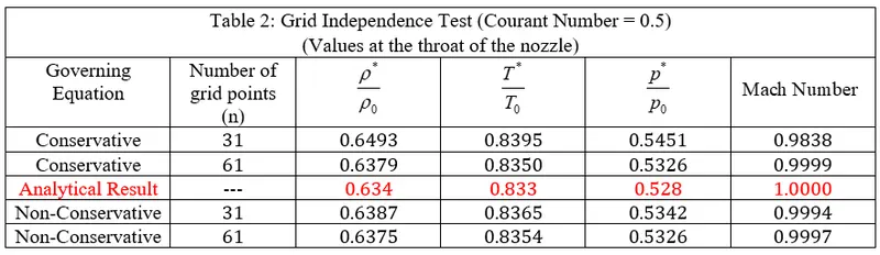
So, it can be observed that on doubling the number of grids there is only a slight improvement in the solution. So in the present study, all the solution plot is obtained using 31 grid points.
MATLAB code:
% Program to solve Quasi 1D flow through convergent divergent nozzle
% Using MacCormack method
% Considering the non-conservative form of governing equation

clear all
close all
clc

% Inputs
n = 31;                                 % Number of grid points
x = linspace(0,3,n);
dx = x(2)-x(1);                         % Grid size
th = ((n+1)/2);                         % Grid point of throat

% Initial conditions
rho = 1-0.3146*x;                       % Non-dimensionalised density
T = 1-0.2314*x;                         % Non-dimensionalised temperature
v = (0.1+1.09*x).*T.^0.5;               % Non-dimensionalised velocity
p = rho.*T;                             % Non-dimensionalised pressure
M = v./T.^0.5;                          % Mach Number

% Area of cross-section
A = 1+2.2*(x-1.5).^2;
mf = rho.*A.*v;                         % Mass flow rate

nt = 1400;                              % Time steps
gamma = 1.4;                            % Ratio of specific heat of air
c = 0.5;                                % CFL number

% Initialising variables for throat location
rho_th = ones(1,nt);
T_th = ones(1,nt);
p_th = ones(1,nt);
M_th = ones(1,nt);

% Outer time loop

for k = 1:nt

    % Creating a copy of primitive variables of previous time step
    rho_old = rho;
    v_old = v;
    t_old = T;

    % Adaptive time step
    for l = 1:n
       dt_1 = (c*dx)/(sqrt(T(l))+v(l));
    end
    dt = min(dt_1);

    % Predictor step

    for j = 2:n-1

        % Calculating spatial derivatives using 1st order accurate forward difference scheme
        dvdx = (v(j+1)-v(j))/dx;
        drhodx = (rho(j+1)-rho(j))/dx;
        dtdx = (T(j+1)-T(j))/dx;
        dlogadx = (log(A(j+1))-log(A(j)))/dx;

        % Continuity equation
        drhodt_p(j) = -rho(j)*dvdx - rho(j)*v(j)*dlogadx -v(j)*drhodx;

        % Momentum equation
        dvdt_p(j) = -v(j)*dvdx - (1/gamma)*(dtdx+(T(j)/rho(j))*drhodx);

        % Energy equation
        dtdt_p(j) = -v(j)*dtdx - (gamma-1)*T(j)*(dvdx + v(j)*dlogadx);

        % Solution update
        rho(j) = rho(j) + drhodt_p(j)*dt;
        v(j) = v(j) + dvdt_p(j)*dt;
        T(j) = T(j) + dtdt_p(j)*dt;
    end

    % Corrector step

    for j = 2:n-1

        % Calculating spatial derivatives using 1st order accurate backward difference scheme
        dvdx = (v(j)-v(j-1))/dx;
        drhodx = (rho(j)-rho(j-1))/dx;
        dtdx = (T(j)-T(j-1))/dx;
        dlogadx = (log(A(j))-log(A(j-1)))/dx;

        % Continuity equation
        drhodt_c(j) = -rho(j)*dvdx - rho(j)*v(j)*dlogadx -v(j)*drhodx;

        % Momentum equation
        dvdt_c(j) = -v(j)*dvdx - (1/gamma)*(dtdx+(T(j)/rho(j))*drhodx);

        % Energy equation
        dtdt_c(j) = -v(j)*dtdx - (gamma-1)*T(j)*(dvdx + v(j)*dlogadx);
    end

    % Calculating the average time derivative
    drhodt = 0.5*(drhodt_p + drhodt_c);
    dvdt = 0.5*(dvdt_p + dvdt_c);
    dtdt = 0.5*(dtdt_p + dtdt_c);

    % Final Solution update

    for i = 2:n-1
       rho(i) = rho_old(i) + drhodt(i)*dt;
       v(i) = v_old(i) + dvdt(i)*dt;
       T(i) = t_old(i) + dtdt(i)*dt;
    end

    % Apply boundary condition

    % Inlet
    v(1) = 2*v(2) - v(3);

    % Outlet
    rho(n) = 2*rho(n-1) - rho(n-2);
    v(n) = 2*v(n-1) - v(n-2);
    T(n) = 2*T(n-1) - T(n-2);

    for i = 1:n
       M(i) = v(i)./(T(i).^0.5);                % Mach number
       mf(i) = rho(i).*A(i).*v(i);              % Mass flow rate
       p(i) = rho(i).*T(i);                     % Pressure
    end

    % Storing values for throat at each time step
    rho_th(k) = rho(th);
    T_th(k) = T(th);
    p_th(k) = p(th);
    M_th(k) = M(th);
    k_th = 1:nt;

%   Plotting mass flow rate at different time steps
%     figure(1)
%     if k == 1
%         plot(x,mf,'-d','LineWidth',1.5)
%         xlim([0 3])
%         ylim([0 2])
%         hold on
%     elseif k == 51
%         plot(x,mf,'LineWidth',1.5)
%         xlim([0 3])
%         ylim([0 2])
%         hold on
%     elseif k == 101
%         plot(x,mf,'LineWidth',1.5)
%         xlim([0 3])
%         ylim([0 2])
%         hold on
%     elseif k == 201
%         plot(x,mf,'LineWidth',1.5)
%         xlim([0 3])
%         ylim([0 2])
%         hold on
%     elseif k == 701
%         plot(x,mf,'LineWidth',1.5)
%         xlim([0 3])
%         ylim([0 2])
%         hold on
%     elseif k == 1001
%         plot(x,mf,'-o','LineWidth',1.5)
%         xlim([0 3])
%         ylim([0 2])
%         hold on
%     elseif k == 1400
%         plot(x,mf,'--','LineWidth',1.5)
%         xlim([0 3])
%         ylim([0 2])
%         hold on
%         legend('0\Deltat','50\Deltat','100\Deltat','200\Deltat','700\Deltat','1000\Deltat','1400\Deltat')
%         xlabel('x/l \rightarrow','FontSize',18);
%         ylabel('{\rhoav}/{{\rho}_0{a}^*{a}_0} \rightarrow','FontSize',16);
%         title('Variation of mass flow rate at different time steps (Non-conservative governing equation)','FontSize',16)
%     end
end

% Importing data at the throat into a .txt file
f1 = fopen('Non_Conservative_31.txt','w');

fprintf(f1,'The value of the non-dimensionalised parameters at the throat of the nozzle\n');
fprintf(f1,'The grid size %d and courant number %f \n\n', n,c);
fprintf(f1,'The Non-Conservative form of equation is solved\n');
fprintf(f1,'%-5s %-8s %-10s %-9s %-11s\n','x/l','Density','Temperature','Pressure','Mach Number');
fprintf(f1,'====  =======  =========== ========  ===========\n');

for m = 1:n
    l(m) = (m-1)*dx;
    fprintf(f1,'%-4.2f    %-3.4f     %-5.4f    %-3.4f     %-5.4f', l(m), rho(m), T(m), p(m), M(m));
    fprintf(f1,'\n');
end
fclose(f1);
%-------------------------------------------------------------------------%


% Plots for time Variation

% subplot(2,2,1)
% plot(k_th,rho_th,'LineWidth',1.5)
% grid on
% title('Variation of density at throat with time-step');
% xlabel('Time Step \rightarrow')
% ylabel('{\rho}/{\rho}_0 \rightarrow')
%
% subplot(2,2,2)
% plot(k_th,T_th,'LineWidth',1.5)
% grid on
% title('Variation of Temperature at throat with time-step');
% xlabel('Time Step \rightarrow')
% ylabel('{T}/{T}_0 \rightarrow')
%
% subplot(2,2,3)
% plot(k_th,p_th,'LineWidth',1.5)
% grid on
% title('Variation of Pressure at throat with time-step');
% xlabel('Time Step \rightarrow')
% ylabel('{p}/{p}_0 \rightarrow')
%
% subplot(2,2,4)
% plot(k_th,M_th,'LineWidth',1.5)
% grid on
% title('Variation of Mach Number at throat with time-step');
% xlabel('Time Step \rightarrow')
% ylabel('M \rightarrow')
%
% suptitle('Variation of parameters with time step for Quasi-1D convergent-divergent nozzle flow (Non-conservative governing equation)')

% Plots showing variation of primitive variables in the computational domain
%
% subplot(3,1,1)
% plot(x,rho,'LineWidth',1.5)
% grid on
% title('Non-Dimensionalised density');
% xlabel('x/l \rightarrow')
% ylabel('{\rho}/{\rho}_0 \rightarrow')
%
% subplot(3,1,2)
% plot(x,M,'LineWidth',1.5)
% grid on
% title('Mach Number');
% xlabel('x/l \rightarrow')
% ylabel('M \rightarrow')
%
% subplot(3,1,3)
% plot(x,T,'LineWidth',1.5)
% grid on
% title('Non-Dimensionalised Temperature');
% xlabel('x/l \rightarrow')
% ylabel('{T}/{T}_0 \rightarrow')
%
% suptitle('Steady state variation of primitive variables for Quasi-1D convergent-divergent nozzle flow (Non-conservative governing equation)')

% PLotting steady state mass flow rate in the domain
% plot(x,mf,'LineWidth',1.5)
% grid on
% title('Mass Flow rate')
% xlabel('x/l \rightarrow','FontSize',16)
% ylabel('Mass Flow Rate \rightarrow','FontSize',16)
% title('Variation of steady state mass flow rate (Non-Conservative governing equation)','FontSize',16)
The plots obtained are as follows:
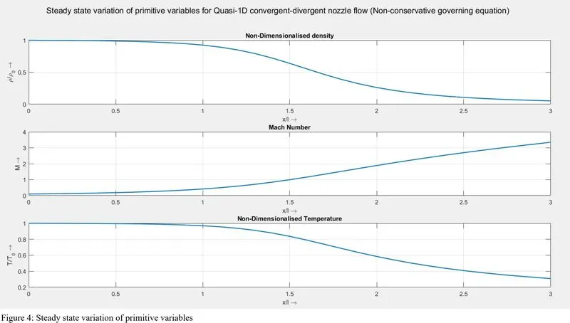
The above plot shows the steady-state variation of the primitive variables. As the present problem is solved for subsonic-supersonic flow in the CD nozzle. So the same can be observed from the plot of Mach number in which the Mach number at the throat is 1.
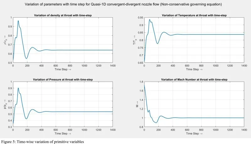
The above plot is the time-wise variation of the primitive variables. The above fluctuation is the numerical fluctuation that occurs as the computation takes place.
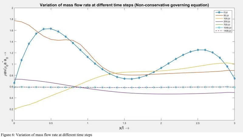
The above plot shows the variation of mass flow rate in the nozzle taken at different time steps. One can notice from the above plot that as the time step proceeds the fluctuation in the mass flow rate decreases and tends to the steady-state solution. This fluctuation is obvious because the mass flow rate is a dependent variable on the primitive variable and the primitive variable itself shows fluctuation in values as time proceeds.
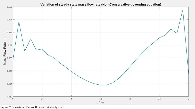
The above plot shows the variation of the mass flow rate in the nozzle at the steady-state. Although there should not be any fluctuation present because this is a constant mass flow rate problem. But when closely observed the plot it can be seen that the fluctuation are very close to the analytic solution which is `dot m = 0.579`
Conservative Governing Equation:
Following are the non-dimensionalized governing equation in the conservative form:
Continuity equation:
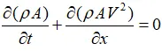
Momentum equation:

Energy equation:

The above set of equations can also be written by defining the solution variable, flux variable, and the source term as follows:
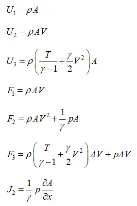
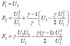
So the above set of governing equations in terms of the solution variable (`U_1, U_2, U_3`), flux variable (`F_1, F_2, F_3`), and source term (`J_2`).
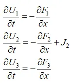
Here, the flux variables are defined in terms of primitive variables. It has been found in studies that when flux variable is defined in terms of primitive variables then the computer program gets blew up. This behavior is an example of a lack of "purity" in the formulation of the governing equations in conservation form, a lack that eventually causes numerical problems. So, the flux variable is written in terms of solution variables (`U_1, U_2, U_3`) in order to avoid that instability.
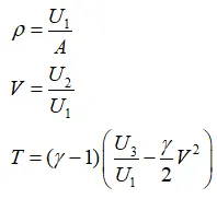
The above set of equations is solved for the solution variable using the MacCormack method and then the primitive variable is calculated from the solution variable using the following relation.
Boundary Condition:
At the subsonic inlet:
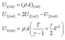
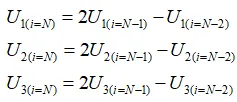
At the supersonic outlet, all the solution variables are extrapolated from the adjacent inner node
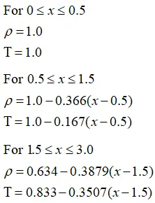
Initial Condition:
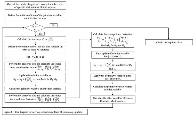
Below a flow diagram is attached showing the solution procedure of conservative form of governing equation using the MATLAB code.
MATLAB Code:
% Quasi-1D supersonic CD nozzle flow simulation
% Solving conservative-form of governing equation
% Using the MacCormack method

clear all
close all
clc

% Inputs
n = 31;                                 % Number of grid points
x = linspace(0,3,n);
dx = x(2)-x(1);                         % Grid size
th = ((n+1)/2);                         % Grid point of throat

nt = 1400;                              % Number of time steps
c = 0.5;                                % CFL number

% Initialisation of variables
l = zeros(1,n);
rho = zeros(1,n);
T = zeros(1,n);
p = zeros(1,n);
F1 = zeros(1,n);
F2 = zeros(1,n);
F3 = zeros(1,n);

% Initialising variables for throat location
rho_th = ones(1,nt);
T_th = ones(1,nt);
p_th = ones(1,nt);
M_th = ones(1,nt);

% Area of cross-section
A = 1+2.2*(x-1.5).^2;
gamma = 1.4;

% Initial condition
for i = 1:n
   l(i) = (i-1)*dx;

   if l(i)<=0.5
      rho(i) = 1.0;
      T(i) = 1.0;
   elseif l(i)>=0.5 && l(i)<=1.5
       rho(i) = 1 - 0.366*(x(i)-0.5);
       T(i) = 1 - 0.167*(x(i)-0.5);
   elseif l(i) >=1.5 && l(i) <=3.0
       rho(i) = 0.634 - 0.3879*(x(i)-1.5);
       T(i) = 0.833 - 0.3507*(x(i)-1.5);
   end
end

v = 0.59./(rho.*A);

% Derived variables
mf = rho.*A.*v;                         % Mass flow rate
M = v./(T);                             % Mach number

% Time loop start
for k = 1:nt

    % Create a copy of primitive variables to store the value of previous
    % time step
    rho_old = rho;
    v_old = v;
    T_old = T;

    % Adaptive time step
    for l = 1:n
       dt_1 = (c*dx)/(sqrt(T(l))+v(l));
    end
    dt = min(dt_1);

    % Defining the solution variables
    U1 = rho.*A;
    U2 = rho.*A.*v;
    U3 = rho.*A.*((T/(gamma-1))+0.5*gamma*v.^2);

    % Create a copy of U1, U2, and U3
    U1_old = U1;
    U2_old = U2;
    U3_old = U3;

    % Defining the flux variables
    F1 = U2;
    F2 = (U2.^2)./U1 + ((gamma-1)/gamma)*(U3 - 0.5*gamma*((U2.^2)./U1));
    F3 = (gamma*U2.*U3)./U1 - 0.5*gamma*(gamma-1)*((U2.^3)./U1.^2);

    % Predictor Step
    % Forward difference scheme for spatial discretization

    for i = 2:n-1
       % Defining the source term
       dAdx(i) = (A(i+1) - A(i))/dx;                                    % Forward differencing
       J2(i) = (1/gamma)*rho(i).*T(i).*dAdx(i);                         % Source term

       % Continuity equation
       dU1dt_p(i) = - (F1(i+1)-F1(i))/dx;

       % Momentum equation
       dU2dt_p(i) = - (F2(i+1)-F2(i))/dx + J2(i);

       % Energy equation
       dU3dt_p(i) = - (F3(i+1)-F3(i))/dx;

       % Update the solution variables
       U1(i) = U1(i) + dU1dt_p(i)*dt;
       U2(i) = U2(i) + dU2dt_p(i)*dt;
       U3(i) = U3(i) + dU3dt_p(i)*dt;
    end

    % Update the primitive variables
    rho = U1./A;
    v = U2./U1;
    T = (gamma-1)*((U3./U1) - (gamma)*0.5*v.^2);
    p = rho.*T;

    % Update the flux variables
    F1 = U2;
    F2 = (U2.^2)./U1 + ((gamma-1)/gamma)*(U3 - 0.5*gamma*((U2.^2)./U1));
    F3 = (gamma*U2.*U3)./U1 - 0.5*gamma*(gamma-1)*((U2.^3)./U1.^2);

    % Corrector Step
    % Backward difference scheme for spatial discretization

    for i = 2:n-1
       % Defining the source term
       dAdx(i) = (A(i) - A(i-1))/dx;                                   % Backward differencing
       J2(i) = (1/gamma)*rho(i).*T(i).*dAdx(i);                         % Source term

       % Continuity equation
       dU1dt_c(i) = - (F1(i)-F1(i-1))/dx;

       % Momentum equation
       dU2dt_c(i) = - ((F2(i)-F2(i-1))/dx) + J2(i);

       % Energy equation
       dU3dt_c(i) = - (F3(i)-F3(i-1))/dx;

    end

    % Calculating the average time derivative
    dU1dt = 0.5*(dU1dt_p+dU1dt_c);
    dU2dt = 0.5*(dU2dt_p+dU2dt_c);
    dU3dt = 0.5*(dU3dt_p+dU3dt_c);

    % Final solution update
    for j = 2:n-1
       U1(j) = U1_old(j) + dU1dt(j)*dt;
       U2(j) = U2_old(j) + dU2dt(j)*dt;
       U3(j) = U3_old(j) + dU3dt(j)*dt;
    end

    % Apply boundary condition

    % Subsonic Inlet
    U1(1) = rho(1)*A(1);
    U2(1) = 2*U2(2) - U2(3);
    U3(1) = U1(1)*((T(1)/(gamma-1)) + 0.5*gamma*v(1)^2);

    % Supersonic outlet
    U1(n) = 2*U1(n-1) - U1(n-2);
    U2(n) = 2*U2(n-1) - U2(n-2);
    U3(n) = 2*U3(n-1) - U3(n-2);

    % Calculating primitive variables
    for i = 1:n
       rho(i) = U1(i)./A(i);
       v(i) = U2(i)./U1(i);
       T(i) = (gamma-1)*((U3(i)./U1(i)) - gamma*0.5*v(i).^2);
       p(i) = rho(i).*T(i);
       M(i) = v(i)./sqrt(T(i));
       mf = rho.*A.*v;                         % Mass flow rate
    end

    % Storing values for throat at each time step
    rho_th(k) = rho(th);
    T_th(k) = T(th);
    p_th(k) = p(th);
    M_th(k) = M(th);
    k_th = 1:nt;

    % Plotting mass flow rate at different time steps
%     figure(1)
%     if k == 1
%         plot(x,mf,'-d','LineWidth',1.5)
%         xlim([0 3])
%         ylim([0 2])
%         hold on
%     elseif k == 51
%         plot(x,mf,'LineWidth',1.5)
%         xlim([0 3])
%         ylim([0 2])
%         hold on
%     elseif k == 101
%         plot(x,mf,'LineWidth',1.5)
%         xlim([0 3])
%         ylim([0 2])
%         hold on
%     elseif k == 201
%         plot(x,mf,'LineWidth',1.5)
%         xlim([0 3])
%         ylim([0 2])
%         hold on
%     elseif k == 701
%         plot(x,mf,'LineWidth',1.5)
%         xlim([0 3])
%         ylim([0 2])
%         hold on
%     elseif k == 1001
%         plot(x,mf,'-o','LineWidth',1.5)
%         xlim([0 3])
%         ylim([0 2])
%         hold on
%     elseif k == 1400
%         plot(x,mf,'--','LineWidth',1.5)
%         xlim([0 3])
%         ylim([0 2])
%         hold on
%         legend('0\Deltat','50\Deltat','100\Deltat','200\Deltat','700\Deltat','1000\Deltat','1400\Deltat')
%         xlabel('x/l \rightarrow','FontSize',18);
%         ylabel('{\rhoav}/{{\rho}_0{a}^*{a}_0} \rightarrow','FontSize',16);
%         title('Variation of mass flow rate at different time steps (Conservative governing equation)','FontSize',16);
%     end
end

% Importing data at the throat into a .txt file
f1 = fopen('Conservative_31.txt','w');

fprintf(f1,'The value of the non-dimensionalised parameters at the throat of the nozzle\n');
fprintf(f1,'The grid size %d and courant number %f \n\n', n,c);
fprintf(f1,'The Conservative form of equation is solved\n');
fprintf(f1,'%-5s %-8s %-10s %-9s %-11s\n','x/l','Density','Temperature','Pressure','Mach Number');
fprintf(f1,'====  =======  =========== ========  ===========\n');

for m = 1:n
    l(m) = (m-1)*dx;
    fprintf(f1,'%-4.2f   %-3.4f     %-5.4f    %-3.4f     %-5.4f', l(m), rho(m), T(m), p(m), M(m));
    fprintf(f1,'\n');
end
fclose(f1);
%-------------------------------------------------------------------------%
%
% % Plots for time Variation

subplot(2,2,1)
plot(k_th,rho_th,'LineWidth',1.5)
grid on
title('Variation of density at throat with time-step');
xlabel('Time Step \rightarrow')
ylabel('{\rho}/{\rho}_0 \rightarrow')
xlim([0 1400])
ylim([0.6 0.7])

subplot(2,2,2)
plot(k_th,T_th,'LineWidth',1.5)
grid on
title('Variation of Temperature at throat with time-step');
xlabel('Time Step \rightarrow')
ylabel('{T}/{T}_0 \rightarrow')
xlim([0 1400])
ylim([0.8 0.86])

subplot(2,2,3)
plot(k_th,p_th,'LineWidth',1.5)
grid on
title('Variation of Pressure at throat with time-step');
xlabel('Time Step \rightarrow')
ylabel('{p}/{p}_0 \rightarrow')
xlim([0 1400])
ylim([0.5 0.6])

subplot(2,2,4)
plot(k_th,M_th,'LineWidth',1.5)
grid on
title('Variation of Mach Number at throat with time-step');
xlabel('Time Step \rightarrow')
ylabel('M \rightarrow')
xlim([0 1400])
ylim([0.97 1.04])

suptitle('Variation of parameters with time step for Quasi-1D convergent-divergent nozzle flow (Conservative governing equation)')

% % Plots showing variation of primitive variables in the computational domain
%
% subplot(3,1,1)
% plot(x,rho,'LineWidth',1.5)
% grid on
% title('Non-Dimensionalised density');
% xlabel('x/l \rightarrow')
% ylabel('{\rho}/{\rho}_0 \rightarrow')
%
% subplot(3,1,2)
% plot(x,M,'LineWidth',1.5)
% grid on
% title('Mach Number');
% xlabel('x/l \rightarrow')
% ylabel('M \rightarrow')
%
% subplot(3,1,3)
% plot(x,T,'LineWidth',1.5)
% grid on
% title('Non-Dimensionalised Temperature');
% xlabel('x/l \rightarrow')
% ylabel('{T}/{T}_0 \rightarrow')
% ylim([0 1])
%
% suptitle('Steady state variation of primitive variables for Quasi-1D convergent-divergent nozzle flow (Conservative governing equation)')

% plot(x,mf,'LineWidth',1.5)
% grid on
% title('Mass Flow rate')
% xlabel('x/l \rightarrow','FontSize',16)
% ylabel('Mass Flow Rate \rightarrow','FontSize',16)
% % ylim([0.582 0.583])
% title('Variation of steady state mass flow rate (Conservative governing equation)','FontSize',16)
The plots obtained by solving the conservative form of governing equation is as follows:
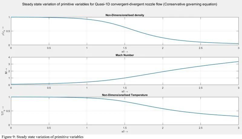
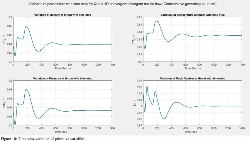
On comparing figures (5) and (10), one can observe that the numerical fluctuation in the primitive variable is more for a non-conservative form of governing equation and the can be observed for the variation of mass flow rate at different time steps, refer to figure (6) and (11).
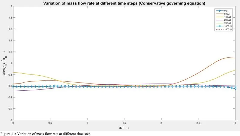
One more reason that the mass flow rate at different time steps is near to the steady-state solution value is that in the conservative form of the governing equation, the equation solves for solution variable and one of the solution variables is itself the mass flow rate.
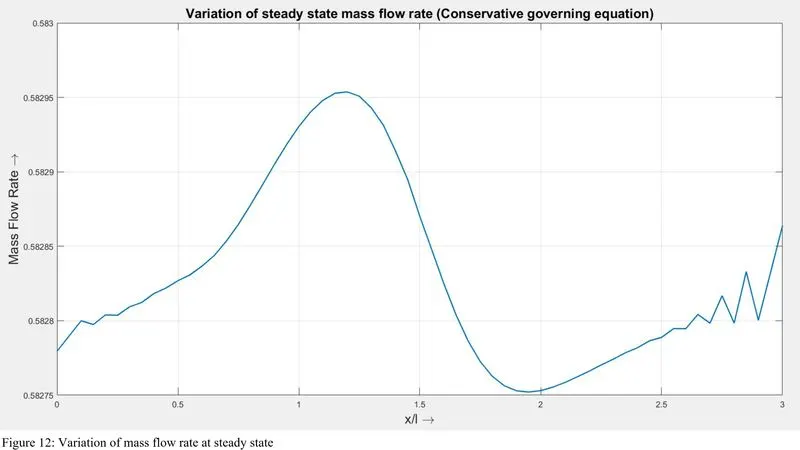
On comparing figures (7) and (12), it can be observed that the fluctuation in the mass flow rate at a steady state is least for the solution of a conservative form of governing equation. Also, the mass flow rate distribution is almost constant as well as closer to the analytical solution.
Conclusion:
1. The conservation form of governing equation gives better mass flow rate distribution at a steady state.
2. Both the form of the governing equation gives satisfactory result but in comparison, the non-conservative form gives slightly better result than the conservative form, refer Table (2).
3. From the computational point of view, the non-conservative form is slightly easier to program because the equations are solved directly in terms of primitive variables while in the conservative form the equations are solved in terms of solution variables and from there the value of primitive variables are obtained.
Both the forms have their own pros and cons and are implemented according to the complexity of the problem and the accuracy of the solution required for the problem.
References:
1. Computational Fluid Dynamics (The basics with Applications), John D. Anderson, Jr. - 1995.
2. Modern Compressible Flow With Historical Perspective, John D. Anderson, Jr. - 3rd Edition, 2003.