Week 9 - FVM Literature Review

Finite Volume Method (FVM) solves the governing equations that describe the flow over a volume instead of a point, irrespective of the shape of the volume which provides an advantage of formulating and working with unstructured meshes in comparison to the finite difference method (FDM). The flow quantities are conserved inside this particular volume. This means that the flow entering the volume will be the same as the flow leaving the volume as far as there isn't a source or sink inside the volume that disrupts this flow.

Firstly, the governing equations are formulated in their integral form and then converted to discretized form with the help of surface integrals obtained from the Gauss-divergence theorem. Since these are surface integrals evaluated on the surfaces of the finite volumes which is obtained by discretizing the entire flow domain, the fluxed entering and leaving these volumes are crucial and are conserved.

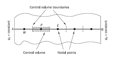
This figure represents the schematic for a sample grid that is generated for solving the governing equations using the finite volume method. Here, it can be observed that the finite volume is the volume that surrounds the grid point or can also be seen as the grid point/point at which the information is stored is at the centre of the discretized finite volume. Hence, they act as the nodes and the boundaries for these volumes have been depicted too.

For example, considering the 1D linear heat conduction equation:

`del/(delx)(alpha.(delT)/(delx))+S=0`

Here,

`alpha` = Thermal Diffusivity

`S`= Source term

`(delT)/(delx)`= Temperature gradient wrt x

Considering the volume integral:

`int(del/(delx)(alpha(delT)/(delx))+S).dV=0`

`intdel/(delx)(alpha(delT)/(delx))dV+intS.dV=0`

We know, `dV=A.dx`

`int_w^edel/(delx)(alpha(delT)/(delx))Adx+intS.dV=0`

`alpha_eA(delT)/(delx_e)-alpha_wA(delT)/(delx_w)+S_(avg)dV=0`

Writing this in the difference form/discretised form gives:

`alphaA((T_E-T_P)/(Deltax))-alphaA((T_P-T_W)/(Deltax))+S_u+S_pT_p=0`

Major differences between FDM & FVM:

• FVM solves the governing equations over a finite volume while the FDM solves the governing equations over a point.
• FDM is not suitable for simulating irregular domain shapes or volumes while on the other hand, FVM can simulate these types of volumes with greater ease.
• FVM equations are comparatively more complex to solve than the FDM equations.
• For FDM the data from the neighbouring points are used for the interpolation methods, while in the FVM the data from the neighbouring faces that are shared by the neighbouring cells/volumes are used for the interpolation.

Need for interpolation schemes in FVM:

The interpolation or the approximation schemes are required in the FVM method for the conversion of the integral form of the governing equation to an algebraic equation which can then be solved using numerical methods. These schemes also play a significant role in the calculation of the values of the flow quantities in the point of concern from the values that are already known from their neighbouring faces/cells. Some of the interpolation schemes can be listed as:

• Upwing interpolation
• Linear interpolation
• QUICK - Quadratic upwind interpolation scheme
• Hybrid scheme

Need for flux limiters in FVM:

These are the limiter values that limit the gradient values when there are very high gradients and discontinuities and function similar to the boundary conditions. These come into relevance for the high-resolution schemes in order to limit the spatial derivatives when solving PDEs.