Week 5.1 - Mid term project - Solving the steady and unsteady 2D heat conduction problem
AIM: To solve the 2D heat conduction equation by using the point iterative techniques for both steady state and transient cases
METHODS FOLLOWED:
Considering the following grid and grid points for the 2D heat conduction problem where T represents temperature at the respective points
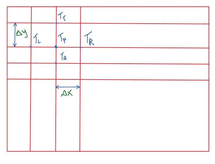
This equally spaced grid represents the 2D domain where the Temperature values are to be calculated and computed. The following methods provide an iterative technique to compute these values from the boundary values provided by the user.
ALGORITHM USED FOR THE CODE:
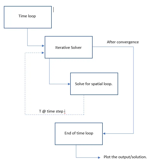
Steady state case:
1. Jacobi method:
For the steady state 2D conduction equation given by: `(partial^2T)/(partialx^2) +(partial^2T)/(partialy^2) = 0`
The solution using jacobi method can be written as,
`T_p^(k+1) = (Deltay^2(T_L^k+T_R^k)+Deltax^2(T_T^k+T_B^k))/(2(Deltax^2+Deltay^2))`
This equation is iterated with the help of neighbouring values of the previous iteration until the error between two consucutive iterations comes down below the set tolerance level. This method is called convergence.
k is the iteration number
2. Gauss-Seidel method:
For the steady state 2D conduction equation given by: `(partial^2T)/(partialx^2) +(partial^2T)/(partialy^2) = 0`
The solution using Gauss seidel method can be written as,
`T_p^(k+1) = (Deltay^2(T_L^(k+1)+T_R^k)+Deltax^2(T_T^(k+1)+T_B^k))/(2(Deltax^2+Deltay^2))`
This is similar toi Jacobi method but instead of considering the neighbouring values from previous iteration here the know values of the current iteration is taken into account and hence reaches faster convergence with lower number of iterations.
k is the iteration number
3. SOR method
For the steady state 2D conduction equation given by: `(partial^2T)/(partialx^2) +(partial^2T)/(partialy^2) = 0`
The solution using SOR method can be written as,
`T_p^(k+1) = (1-omega)*T_p^(k) + omega.(Deltay^2(T_L^(k+1)+T_R^k)+Deltax^2(T_T^(k+1)+T_B^k))/(2(Deltax^2+Deltay^2))`
This method uses a relazation factor `omega` that helps in controlling how the convergence can be varied by either scaling it up or down that can lead to faster convergence in particular cases.
k is the iteration number
CODE:
clear all
close all
clc

% inputs
nx = 10;
ny = 10;
omega = 1.1;

% initialization and boundary conditions
T = 300*ones(nx,ny);
T(1,2:end-1) = 600;
T(end,2:end-1) = 900;
T(2:end-1,1) = 400;
T(2:end-1,end) = 800;
T(1,1) = (T(1,2) + T(2,1))/2;
T(end,end) = (T(end,end-1) + T(end-1,end))/2;
T(end,1) = (T(end-1,1) + T(end,2))/2;
T(1,end) = (T(1,end-1) + T(2,end))/2;

% creating a copy of T
T_old = T;
x = linspace(0,1,nx);
dx = x(2) - x(1);
y = linspace(0,1,ny);
dy = y(2) - y(1);

k = 2*((dx^2+dy^2)/(dx^2*dy^2));
method = 3;
error = 1e3;
tol = 1e-4;

% jacobi method
if (method == 1)
    jacobi_iter = 1;
    while (error>tol)

        for i = 2:nx-1
            for j = 2:ny-1
                term1 = (T_old(i-1,j)+T_old(i+1,j))/(dx^2*k);
                term2 = (T_old(i,j-1)+T_old(i,j+1))/(dy^2*k);
                T(i,j) = term1 + term2;
            end
        end

        error = max(max(abs(T_old - T)));
        T_old = T;
        jacobi_iter = jacobi_iter + 1;

        %plotting
        [A,B] = contourf(x,y,T);
        clabel(A,B)
        colormap(jet);
        colorbar;
        title_text = sprintf('Iteration number = %d',jacobi_iter);
        title(title_text)
        xlabel('X axis');
        ylabel('Y axis');
        set(gca,'YDIR','reverse');
        pause(0.03)

    end
end

% gauss-siedel method
if (method == 2)
    GS_iter = 1;
    while (error>tol)

        for i = 2:nx-1
            for j = 2:ny-1
                term1 = (T(i-1,j)+T_old(i+1,j))/(dx^2*k);
                term2 = (T(i,j-1)+T_old(i,j+1))/(dy^2*k);
                T(i,j) = term1 + term2;
            end
        end

        error = max(max(abs(T_old - T)));
        T_old = T;
        GS_iter = GS_iter + 1;

        %plotting
        [A,B] = contourf(x,y,T);
        clabel(A,B)
        colormap(jet);
        colorbar;
        title_text = sprintf('Iteration number = %d',GS_iter);
        title(title_text)
        xlabel('X axis');
        ylabel('Y axis');
        set(gca,'YDIR','reverse');
        pause(0.03)

    end
end

% SOR method
if (method == 3)
    SOR_iter = 1;
    while (error>tol)

        for i = 2:nx-1
            for j = 2:ny-1
                term1 = (T(i-1,j)+T_old(i+1,j))/(dx^2*k);
                term2 = (T(i,j-1)+T_old(i,j+1))/(dy^2*k);
                T(i,j) = (1-omega)*T_old(i,j) + omega*(term1 + term2);
            end
        end

        error = max(max(abs(T_old - T)));
        T_old = T;
        SOR_iter = SOR_iter + 1;

        % plotting
        [A,B] = contourf(x,y,T);
        clabel(A,B)
        colormap(jet);
        colorbar;
        title_text = sprintf('Iteration number = %d',SOR_iter);
        title(title_text)
        xlabel('X axis');
        ylabel('Y axis');
        set(gca,'YDIR','reverse');
        pause(0.03)

    end
end
RESULTS:
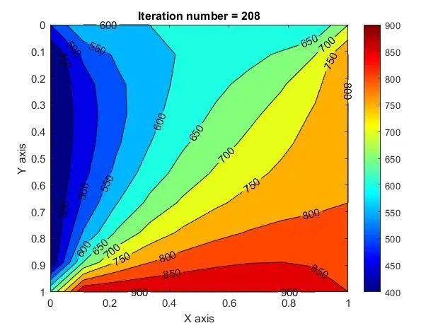
Jacobi method:
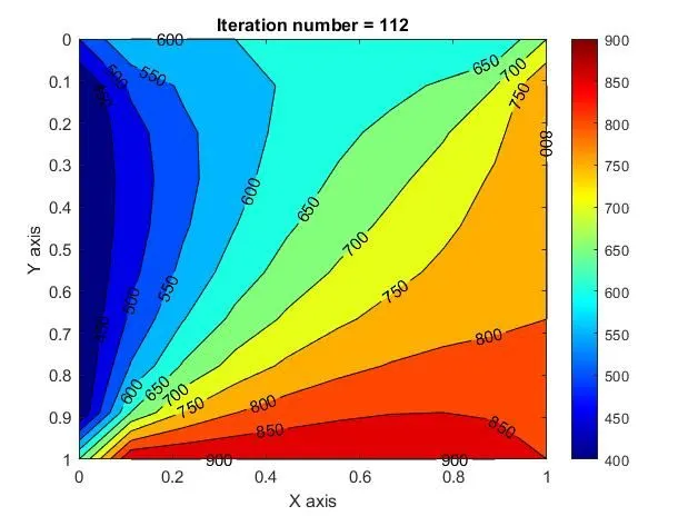
Guass Seidel method:
SOR method:
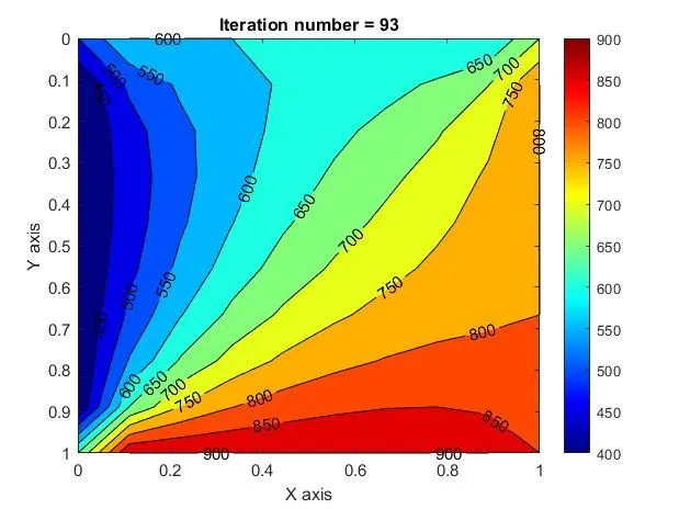
From the above contours it can be observed that the results are same, but only difference with each of the methods is the number of iterations it takes to achieve these results and hence the order can be in Jacobi > GS >SOR, due to the updation and election of values that are used for consecutive iterations
Transient case:
1. Explicit scheme
For the transient case along with iteration number there comes into consideration the variable with respect to time, which is time step size and number of time steps. For the steady state 2D conduction equation given by:
`(partial T)/(partial t) = alpha.((partial^2T)/(partialx^2) +(partial^2T)/(partialy^2))`
The explicit solution is given by:
`(T_p^(n+1)-T_p^n)/(Deltat) = alpha.((T_L-2T_P+T_R)/(Deltax^2) + (T_T-2T_P+T_B)/(Deltay^2))`
hence, this equation can be directly solved by looping over the spatial grid for all the grid points. Here, after rearranging and simplifying we get two constants `k_1` and `k_2` that are called as the CFL numbers which are defined as follows:
`k_1 = alpha.(Deltat)/(Deltax^2)` and `k_2 = alpha.(Deltat)/(Deltay^2)`
These numbers are to be kept less that 0.5 in order for the solution to converge and produce meaningful results. hence it depends on the thermal diffusion coefficient, time step size and grid spacing size.
CODE:
clear all
close all
clc

% inputs
nx = 10;
ny = 10;
alpha = 1.5;

% initialization and boundary conditions
T = 300*ones(nx,ny);
T(1,2:end-1) = 600;
T(end,2:end-1) = 900;
T(2:end-1,1) = 400;
T(2:end-1,end) = 800;
T(1,1) = (T(1,2) + T(2,1))/2;
T(end,end) = (T(end,end-1) + T(end-1,end))/2;
T(end,1) = (T(end-1,1) + T(end,2))/2;
T(1,end) = (T(1,end-1) + T(2,end))/2;

% creating a copy of T
T_old = T;
x = linspace(0,1,nx);
dx = x(2) - x(1);
y = linspace(0,1,ny);
dy = y(2) - y(1);
dt = 2/1400;

k1 = (alpha*dt)/(dx^2);
k2 = (alpha*dt)/(dy^2);

% explicit method

for nt = 1:1400
    for i = 2:nx-1
        for j = 2:ny-1
            term1 = T_old(i,j);
            term2 = k1*(T_old(i+1,j)-2*T_old(i,j)+T_old(i-1,j));
            term3 = k2*(T_old(i,j+1)-2*T_old(i,j)+T_old(i,j-1));
            T(i,j) = term1 + term2 + term3;
        end
    end
    T_old = T;

    %plotting
    [A,B] = contourf(x,y,T);
    clabel(A,B)
    colormap(jet);
    colorbar;
    title_text = sprintf('Explicit method');
    title(title_text)
    xlabel('X axis');
    ylabel('Y axis');
    pause(0.03)

end
RESULT:
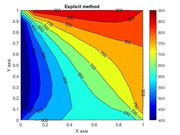
2. Implicit scheme
Again the methods used for steady state simulation can be used to solve the equation iteratively.
a) Jacobi method:
The solution equation after simplifying can be written as a set of following equations:
`k_1 = alpha.(Deltat)/(Deltax^2)` and `k_2 = alpha.(Deltat)/(Deltay^2)`
`term1 = 1/(1+2k_1+2k_2)`, `term2 = k_1*term1` and `term3 = k_2*term1`
The tempreature at time step (n+1) can be calculated from the time step values and n and n+1 using :
`T_p^(n+1) = term1*T_p^n + term2*(T_L+T_R)^(n+1)+term3*(T_T+T_B)^(n+1)`
All the values are considered from the previous iteration.
b) Gauss-Seidel method
The solution equation after simplifying can be written as a set of following equations:
`k_1 = alpha.(Deltat)/(Deltax^2)` and `k_2 = alpha.(Deltat)/(Deltay^2)`
`term1 = 1/(1+2k_1+2k_2)`, `term2 = k_1*term1` and `term3 = k_2*term1`
The tempreature at time step (n+1) can be calculated from the time step values and n and n+1 using :
`T_p^(n+1) = term1*T_p^n + term2*(T_L+T_R)^(n+1)+term3*(T_T+T_B)^(n+1)`
Here known values are considered from the current iteration.
c) SOR method
The solution equation after simplifying can be written as a set of following equations:
`k_1 = alpha.(Deltat)/(Deltax^2)` and `k_2 = alpha.(Deltat)/(Deltay^2)`
`term1 = 1/(1+2k_1+2k_2)`, `term2 = k_1*term1` and `term3 = k_2*term1`
The tempreature at time step (n+1) can be calculated from the time step values and n and n+1 using :
`T_p^(n+1) = (1-omega)*T_P+ omega*(term1*T_p^n + term2*(T_L+T_R)^(n+1)+term3*(T_T+T_B)^(n+1))`
CODE:
clear all
close all
clc

% inputs
nx = 20;
ny = 20;
omega = 1.1;
alpha = 1.5;
dt = 0.1;
t = 100;

% initialization and boundary conditions
T = 300*ones(nx,ny);
T(1,2:end-1) = 600;
T(end,2:end-1) = 900;
T(2:end-1,1) = 400;
T(2:end-1,end) = 800;
T(1,1) = (T(1,2) + T(2,1))/2;
T(end,end) = (T(end,end-1) + T(end-1,end))/2;
T(end,1) = (T(end-1,1) + T(end,2))/2;
T(1,end) = (T(1,end-1) + T(2,end))/2;

% creating a copy of T
T_old = T;
T_prev_dt = T_old;
x = linspace(0,1,nx);
dx = x(2) - x(1);
y = linspace(0,1,ny);
dy = y(2) - y(1);

k1 = alpha*dt/dx^2;
k2 = alpha*dt/dy^2;
method = 3;
tol = 1e-4;

term1 = (1+(2*k1)+(2*k2))^-1;
term2 = k1*term1;
term3 = k2*term1;

% jacobi method
if (method == 1)
    jacobi_iter = 1;
    for n = 1:t/dt
        error =10;
        while error>tol

            for i = 2:nx-1
                for j = 2:ny-1
                    H = (T_old(i-1,j) + T_old(i+1,j));
                    V = (T_old(i,j-1) + T_old(i,j+1));
                    T(i,j) = (T_prev_dt(i,j)*term1) + (H*term2) + (V*term3);
                end
            end

            error = max(max(abs(T_old-T)));
            jacobi_iter = jacobi_iter + 1;
            T_old = T;

        end
        T_prev_dt = T;

    end

        %plotting
        [A,B] = contourf(x,y,T);
        clabel(A,B)
        colormap(jet);
        colorbar;
        title_text = sprintf('time steps = %d Jacobi terations = %d',n,jacobi_iter);
        title(title_text)
        xlabel('X axis');
        ylabel('Y axis');
        set(gca,'YDIR','reverse');
end

% gauss seidel method
if (method == 2)
    GS_iter = 1;
    for n = 1:t/dt
        error =10;
        while error>tol

            for i = 2:nx-1
                for j = 2:ny-1
                    H = (T(i-1,j) + T_old(i+1,j));
                    V = (T(i,j-1) + T_old(i,j+1));
                    T(i,j) = (T_prev_dt(i,j)*term1) + (H*term2) + (V*term3);
                end
            end

            error = max(max(abs(T_old-T)));
            GS_iter = GS_iter + 1;
            T_old = T;

        end
        T_prev_dt = T;

    end

        %plotting
        [A,B] = contourf(x,y,T);
        clabel(A,B)
        colormap(jet);
        colorbar;
        title_text = sprintf('time steps = %d GS iterations = %d',n,GS_iter);
        title(title_text)
        xlabel('X axis');
        ylabel('Y axis');
        set(gca,'YDIR','reverse');
end

% SOR method
if (method == 3)
    SOR_iter = 1;
    for n = 1:t/dt
        error =10;
        while error>tol

            for i = 2:nx-1
                for j = 2:ny-1
                    H = (T(i-1,j) + T_old(i+1,j));
                    V = (T(i,j-1) + T_old(i,j+1));
                    T(i,j) = (1-omega)*T_old(i,j) + omega*((T_prev_dt(i,j)*term1) + (H*term2) + (V*term3));
                end
            end

            error = max(max(abs(T_old-T)));
            SOR_iter = SOR_iter + 1;
            T_old = T;

        end
        T_prev_dt = T;

    end

        %plotting
        [A,B] = contourf(x,y,T);
        clabel(A,B)
        colormap(jet);
        colorbar;
        title_text = sprintf('time steps = %d SOR iteration = %d',n,SOR_iter);
        title(title_text)
        xlabel('X axis');
        ylabel('Y axis');
        set(gca,'YDIR','reverse');
end
RESULTS:
Jacobi method:
Gauss Siedel method:
SOR method:
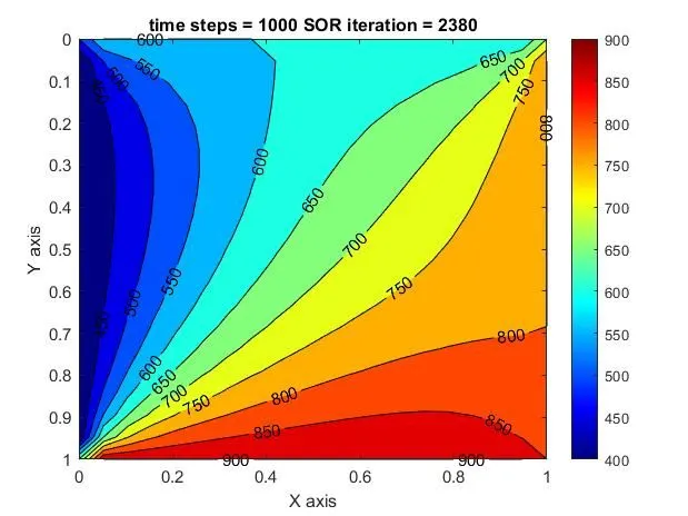
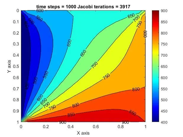
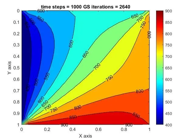
Similarly for the unsteady case, from the above contours it can be observed that the results are same, but only difference with each of the methods is the number of iterations it takes to achieve these results and hence the order can be in Jacobi > GS >SOR, due to the updation and election of values that are used for consecutive iterations.