Week 3.5 - Deriving 4th order approximation of a 2nd order derivative using Taylor Table method

AIM: To generate a plot comparing the different schemes such as the central differencing, left-skewed, and right-skewed schemes for deriving 4th order approximation of a 2nd order derivative using the Taylor Table method.

GIVEN DATA:

`f(x) = e^x.cos(x)`

Analytical solution:

`f''(x) = -2e^xsin(x)`

The expression for central difference scheme of 4th order approximation for a 2nd order derivative can be written as:

`f''(x) = (a*f(x-2h)+ b*f(x-h)+ c*f(x) +d*f(x+h) + e*f(x+2h))/h^2`

The expression for left-skewed scheme of 4th order approximation for a 2nd order derivative can be written as:

`f''(x) = (a*f(x)+ b*f(x-h)+ c*f(x-2h) +d*f(x-3h) + e*f(x-4h) + g*f(x-5h))/h^2`

The expression for right-skewed scheme of 4th order approximation for a 2nd order derivative can be written as:

`f''(x) = (a*f(x)+ b*f(x+h)+ c*f(x+2h) +d*f(x+3h) + e*f(x+4h) + g*f(x+gh))/h^2`

SOLUTION:

Right-skewed scheme:

For the Taylor's table method a Hypothesis function can be written as:

`(partial^2u)/(partialx^2) = a*f(i) + b*f(i+1) + c*f(i+2) + d*f(i+3) + e*f(i+4) + g*f(i+5)`

TT	`f(i)`	`Delta x*f'(i)`	`Delta x^2*f''(i)`	`Delta x^3*f'''(i)`	`Delta x^4*f^(IV)(i)`	`Delta x^5*f^(V)(i)`	`Delta x^6*f^(VI)(i)`
`a*f(i)`	a	0	0	0	0	0	0
`b*f(i+1)`	b	b	b/2	b/6	b/24	b/120	b/720
`c*f(i+2)`	c	2c	4c/2	8c/6	16c/24	32c/120	64c/720
`d*f(i+3)`	d	3d	9d/2	27d/6	81d/24	243d/120	729d/720
`e*f(i+4)`	e	4e	16e/2	64e/6	256e/24	1024e/120	4096e/720
`g.f(i+5)`	g	5g	25g/2	125g/6	625g/24	3125g/120	15625g/720
`(partial^2u)/(partialx^2)`	0	0	1	0	0	0	?

Hence, this table can be converted into a matrix and solved in Matlab in the following format:

A.X = B

`[[1, 1, 1, 1, 1, 1],[0, 1, 2, 3, 4, 5],[0, 1/2, 2, 9/2, 16/2, 25/2],[0, 1/6, 8/6, 27/6, 64/6, 125/6],[0, 1/24, 16/24, 81/24, 256/24, 1024/24],[0, 1/120, 32/120, 243/120, 1024/120, 3125/120]].[[a],[b],[c],[d],[e],[f],[g]] = [[0],[0],[1],[0],[0],[0]]`

This is a system of algebraic equations that can be solved to obtain the values of a,b,c,d,e as a vector in MATLAB

After obtaining the values of these unknown variables they can be substituted in the hypothesized function to obtain the approximation. This approximated value is then subtracted with the analytical solution to obtain the error for the right-skewed scheme.

Left-skewed scheme:

For the Taylor's table method a Hypothesis function can be written as:

`(partial^2u)/(partialx^2) = a*f(i-5) + b*f(i-4) + c*f(i-3) + d*f(i-2) + e*f(i-1) + g*f(i)`

TT	`f(i)`	`Delta x*f'(i)`	`Delta x^2*f''(i)`	`Delta x^3*f'''(i)`	`Delta x^4*f^(IV)(i)`	`Delta x^5*f^(V)(i)`	`Delta x^6*f^(VI)(i)`	`Delta x^7*f^(VII)(i)`
`a*f(i-5)`	a	-5.a	25a/2	-125a/6	625a/24	-3125a/120	15625a/240
`b*f(i-4)`	b	-4b	16b/2	-64b/6	256b/24	-1024b/120	4096b/240
`c*f(i-3)`	c	-3c	9c/2	-27c/6	81c/24	-243c/120	729c/240
`d*f(i-2)`	d	-2d	4d/2	-8d/6	16d/24	-32d/120	64d/240
`e*f(i-1)`	e	-e	e/2	-e/6	e/24	-e/120	e/240
`g.f(i)`	g	0	0	0	0	0	0
`(partial^2u)/(partialx^2)`	0	0	1	0	0	?	?

Hence, this table can be converted into a matrix and solved in Matlab in the following format:

A.X = B

`[[1, 1, 1, 1, 1, 1],[-5, -4, -3, -2, -1, 0],[25/2, 16/2, 9/2, 2, 1/2, 0],[-125/6, -64/6, -27/6, -8/6, -1/6, 0],[625/24, 256/24, 81/24, 16/24, 1/24, 0],[-3125/120, -1024/120, -243/120, -32/120, -1/120, 0]].[[a],[b],[c],[d],[e],[f],[g]] = [[0],[0],[1],[0],[0],[0]]`

This is a system of algebraic equations that can be solved to obtain the values of a,b,c,d,e as a vector in MATLAB

After obtaining the values of these unkown variables they can be substituted in the hypothesised function to obtain the approximation. This approximated value is then subtracted with the analytical solution to obtain the error for left skewed scheme.

Central difference scheme:

For the Taylor's table method a Hypothesis function can be written as:

`(partial^2u)/(partialx^2) = a*f(i-2) + b*f(i-1) + c*f(i) + d*f(i+1) + e*f(i+2)`

TT	`f(i)`	`Delta x*f'(i)`	`Delta x^2*f''(i)`	`Delta x^3*f'''(i)`	`Delta x^4*f^(IV)(i)`	`Delta x^5*f^(V)(i)`	`Delta x^6*f^(VI)(i)`
`a*f(i-2)`	a	-2.a	4a/2	-8a/6	16a/24	-32a/120	64a/240
`b*f(i-1)`	b	-b	b/2	-b/6	b/24	-b/120	b/240
`c*f(i)`	c	-3c	0	0	0	0	0
`d*f(i+1)`	d	-2d	d/2	d/6	d/24	d/120	d/240
`e*f(i+2)`	e	2e	4e/2	8e/6	16e/24	32e/120	64e/240
`(partial^2u)/(partialx^2)`	0	0	1	0	0	?	?

Hence, this table can be converted into a matrix and solved in Matlab in the following format:

A.X = B

`[[1, 1, 1, 1, 1],[-2, -1, 0, 1, 2],[2, 1/2, 0, 1/2, 4/2],[-8/6, -1/6, 0, 1/6, 8/6],[6/24, 1/24, 0, 1/24, 16/24]]. [[a],[b],[c],[d],[e]] = [[0],[0],[1],[0],[0]]``

This is a system of algebraic equations that can be solved to obtain the values of a,b,c,d,e as a vector in MATLAB

After obtaining the values of these unkown variables they can be substituted in the hypothesised function to obtain the approximation. This approximated value is then subtracted with the analytical solution to obtain the error for central difference scheme

CODE:

Main program: The main program contains 2 sections, one for the generation of error values by calling the external functions and the other for plotting these values with respect to the discretization scheme used.

clear all
close all
clc

x = pi/3;
dx = linspace(pi/4, pi/4000, 40);

% For loop to generate an array and store the values from functions
for i = 1:length(dx)

    % fourth order approximation central scheme
    CD_error(i) = central_differencing_scheme(x,dx(i));
    
    % fourth order approximation left skewed
    LS_error(i) = left_skewed_scheme(x,dx(i));
    
    % fourth order approximation right skewed
    RS_error(i) = right_skewed_scheme(x,dx(i));

end

% Plotting in log-log plot for comparison
figure(1)
loglog(dx, CD_error)
hold on
loglog(dx, LS_error)
hold on
loglog(dx, RS_error)
title('Comparison of 4th order approximation of a 2nd order derivative')
legend('central differencing','left skewed','right skewed')
xlabel('dx')
ylabel('Error')

Function for central difference scheme: This code uses an external function f to evaluate the central difference

function out = central_differencing_scheme(x, dx)

% analytical function = (e^x)*cos(x)

% analytical derivative
% f''(x) = -2*sin(x)*e^x

analytical_derivative = -2*sin(x)*exp(x);

% numerical derivative
% fourth order approximation of 2nd derivative
% central differencing scheme - hypothesis function
% (a*f(x-2h)+ b*f(x-h)+ c*f(x) +d*f(x+h) + ef(x+2h))/h^2

% the constants a,b,c,d,e,f are determined using taylors table method
% solved using a matix
%[coefficients]*[variables] = [constants]

%coefficient matrix obtained from taylor's table
coefficient = [1, 1, 1, 1, 1; 
               -2, -1, 0, 1, 2;
               2, 1/2, 0, 1/2, 4/2; 
               -8/6, -1/6, 0, 1/6, 8/6; 
               16/24, 1/24, 0, 1/24, 16/24];
           
constant = [0; 0; 1; 0; 0];

% a,b,c,d,e determined for the hypothesis function
variable = linsolve(coefficient,constant);
a = variable(1);  b = variable(2); c = variable(3); d = variable(4); e = variable(5);

% Fourth order approximation using external function - f
fourth_order_differencing = (a*f(x-(2*dx))+ b*f(x-dx)+ c*f(x) +d*f(x+dx) + e*f(x+(2*dx)))/(dx)^2;

% error_second_order 
out = abs(fourth_order_differencing - analytical_derivative);

end

Function for left-skewed scheme: This code uses an external function f to evaluate the left skewed

function out = left_skewed_scheme(x, dx)

% analytical function = (e^x)*cos(x)

% analytical derivative
% f''(x) = -2*sin(x)*e^x

analytical_derivative = -2*sin(x)*exp(x);

% numerical derivative
% fourth order approximation of 2nd derivative
% left skewed scheme - hypothesis function
% (a*f(x)+ b*f(x-h)+ c*f(x-2h) +d*f(x-3h) + e*f(x-4h) + g*f(x-5h))/h^2

% the constants a,b,c,d,e,f are determined using taylors table method
% solved using a matix
%[coefficients]*[variables] = [constants]

%coefficient matrix obtained from taylor's table
coefficient = [1, 1, 1, 1, 1, 1; 
               -5, -4, -3, -2, -1, 0;
               25/2, 16/2, 9/2, 2, 1/2, 0;        
               -125/6, -64/6, -27/6, -8/6, -1/6, 0;
               625/24, 256/24, 81/24, 16/24, 1/24, 0;
               -3125/120, -1024/120, -243/120, -32/120, -1/120, 0];
           
constant = [0; 0; 1; 0; 0; 0];

% a,b,c,d,e determined for the hypothesis function
variable = linsolve(coefficient,constant);
a = variable(1);  b = variable(2); c = variable(3); d = variable(4); e = variable(5); g = variable(6);

% Fourth order approximation using external function - f
fourth_order_differencing = (a*f(x)+ b*f(x-dx)+ c*f(x-2*dx) +d*f(x-3*dx) +e*f(x-4*dx) +g*f(x-5*dx))/(dx)^2;

% error_second_order 
out = abs(fourth_order_differencing - analytical_derivative);

end

Function for right-skewed scheme: This code uses an external function f to evaluate the right skewed

function out = right_skewed_scheme(x, dx)

% analytical function = (e^x)*cos(x)

% analytical derivative
% f''(x) = -2*sin(x)*e^x

analytical_derivative = -2*sin(x)*exp(x);

% numerical derivative
% fourth order approximation of 2nd derivative
% central differencing scheme - hypothesis function
% (a*f(x)+ b*f(x+h)+ c*f(x+2h) +d*f(x+3h) + e*f(x+4h) + g*f(x+gh))/h^2

% the constants a,b,c,d,e,f are determined using taylors table method
% solved using a matix
%[coefficients]*[variables] = [constants]

%coefficient matrix obtained from taylor's table
coefficient = [1, 1, 1, 1, 1, 1; 
               0, 1, 2, 3, 4, 5;
               0, 1/2, 2, 9/2, 16/2, 25/2; 
               0, 1/6, 8/6, 27/6, 64/6, 125/6; 
               0, 1/24, 16/24, 81/24, 256/24, 1024/24;
               0, 1/120, 32/120, 243/120, 1024/120, 3125/120];
           
constant = [0; 0; 1; 0; 0; 0];

% a,b,c,d,e determined for the hypothesis function
variable = linsolve(coefficient,constant);
a = variable(1);  b = variable(2); c = variable(3); d = variable(4); e = variable(5); g = variable(6);

% Fourth order approximation using external function - f
fourth_order_differencing = (a*f(x)+ b*f(x+dx)+ c*f(x+2*dx) +d*f(x+3*dx) + e*f(x+4*dx) + g*f(x+5*dx))/(dx)^2;

% error_second_order 
out = abs(fourth_order_differencing - analytical_derivative);

end

RESULTS:

A plot comparing these schemes is obtained as follows:

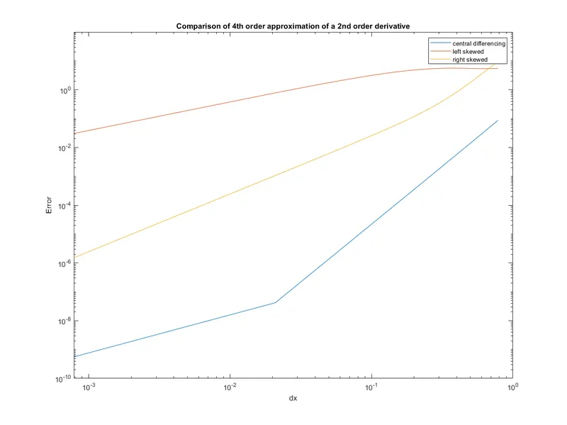
From this, it can be inferred that the central difference scheme has better accuracy than the left and right-skewed schemes. But in tools like CFD central difference scheme cannot be extensively used because the data of both the neighboring points i.e before and after the point is seldom known. Hence a skewed scheme proves useful as only the data in a single direction can help in reaching the required accuracy.