Week 11 - Simulation of Flow through a pipe in OpenFoam
AIM:
To simulate an axisymmetric flow by applying the wedge boundary condition through a pipe in OpenFOAM
GIVEN DATA:
Flow properties that are considered for simulation obey the Hagen-Poisuelle flow equation. The flow is laminar, incompressible, along the length of the pipe, and flows through a constant cross-section pipe at an inlet Reynold's number of 2100. A transient simulation will be performed and the results obtained will be validated with the analytical result from the Hagen-Poisuelle equations.
DATA FROM LITERATURE:
The Hagen-Poisuelle equation is the equation that describes the Hagen-Poisuelle flow, it essentially gives the pressure drop in an incompressible and Newtonian fluid flow that is laminar in nature, this flow can be described as the flow of fluid through a long cylindrical pipe of constant cross-section area. The following assumptions are valid while the equation is defined:
- Fluid is incompressible
- Newtonian fluid
- Flow is laminar
- The dimension defining the length is significantly larger than the diameter of the pipe
When the above assumptions/conditions are met the Hagen-Poisuelle equation defines the pressure drop along with the flow which is essentially due to the viscosity of the fluid. The numerical form of this equation is as follows:
`Deltap=(8muLQ)/(piR^4)`
where:
`Deltap` is the pressure difference between the 2 locations
`L` is the length of the pipe
`mu` is the dynamic viscosity
`Q` is the volumetric flow rate
`R` is the pipe radius
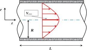
The above image indicates the flow profile developed inside the cylindrical pipe that best represents the Hagen-Poisuelle flow and defined by the Hagen-Poisuelle equations, where the flow develops solely due to the pressure difference established between 2 points before and after the profile zone. The `V_max` indicated the maximum velocity along the centreline of the pipe, and other variables are represented as defined previously in the equation.
Using this concept and available analytical and numerical data/inputs, a simulation of the Hagen-Poisuielle flow is performed with the help of OpenFOAM version 8 and the results have been validated with respect to the analytical solution.
Some of the variables essential for validation of the numerical simulation can be calculated using the following analytical equations:
The Hydro-dynamic length is defined as the length from the inlet face at which the flow reaches the fully developed condition, this can be analytically calculated using the equation,
`L_h = 0.06*D*R_e`
where,
`L_h` = Hydrodynamic length
`D` = Diameter of the pipe
`R_e`= Reynolds number for the flow
The average velocity can be calculated using:
`U_(avg) = (R_emu)/(rhoD)`
The velocity variation along the radius can be given by:
`U(r) = 2*U_(avg).(1-r^2/R^2)`
where,
`r` is the radius variable
`R` is the maximum radius value of the pipe
The pressure drop along the length of the pipe can be analytically calculated using the equation:
`Deltap=(32muLU_(avg))/D^2`
The wall shear stress can be analytically calculated using:
Darcy friction factor: `f = 64/(R_e)`
`tau_w = f/4.(rhoU_(avg)^2)/2`
where `tau_w` is the wall shear stress that the fluid applies on the wall while flowing along the length of the pipe
The values obtained for the above-mentioned parameters have then been used for validating the numerical simulation.
METHODOLOGY FOLLOWED:
For the numerical simulation in the OpenFOAM software, an axisymmetric wedge has been considered as the domain for simulation and respective suitable boundary conditions have been applied in order to simulate the flow as accurately as possible with minimum assumptions.
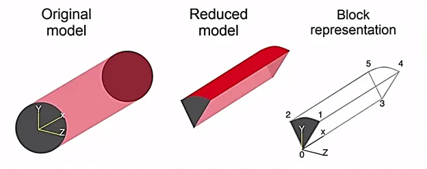
source: skill-lync
The steps are as follows:
- Generation of blockMeshDict file that generates the required domain and meshes this domain
- the blockMeshDict file consists of patches and edges that define the domain inclusive of inlet, outlet, wall, left and right along with the edge for centreline.
- Input dimensions are given to be: Diameter = 0.01m, Length = 3m, wedge angle = 5 degrees
- number of cells along x = 200
- number of cells along y = 20
- number of cells along z = 1
- Grading factor for x = 1
- Grading factor for y = 0.2
- Grading factor for z = 1
- Application of suitable boundary conditions
- inlet: constant velocity inlet calculated from Reynolds number `U = (R_emu)/(rhoD) = 0.1873 m/s`
- outlet: constant pressure outlet `p = 0 (m^2/s^2)` kinematic pressure
- wall: no-slip wall
- left and right: wedge boundary condition the defines axis-symmetric BC
- edge: empty BC that defines the axis for the cylinder
- Definition of constants governing the transport phenomenon
- since its incompressible flow phenomenon, only viscosity is defined
- Set up of simulation parameters in controlDict file and running the simulation
- icoFoam solver is suitable for the given flow type simulation and hence this is used
- the time period for simulation calculated with respect to the length and flow velocity `T = L/U ~ 20s`
- time step size calculated from the CFL number keeping it less than 1 `CFL = (U.Deltat)/(Deltax) <= 1``Deltat = 5e-4`
SIMULATION:
The function in MATLAB generates the blockMeshDict file with the inputs for Diameter of pipe, length of pipe, and wedge angle for the pipe. The generated blockMeshDict file with the given inputs along with the number of cells in each direction and the grading factor is as follows:
/*------------------------------*C++*-------------------------------*
=========                |
\\      / F ield         | OpenFOAM: The Open Source CFD Toolbox
 \\    /  O peration     | Website: https://openfoam.org
  \\  /   A nd           | Version: 8
   \\/    M anipulation  |
*-------------------------------------------------------------------*/
FoamFile
{
	version    2.0;
	format     ascii;
	class      dictionary;
	object     blockMeshDict;
}
//******************************************************************//

convertToMeters 1;

vertices
(
	(0.000000 0.000000 0.000000)
	(0.000000 0.004997 0.000174)
	(0.000000 0.004997 -0.000174)
	(3.000000 0.000000 0.000000)
	(3.000000 0.004997 0.000174)
	(3.000000 0.004997 -0.000174)
);

blocks
(
	 hex (0 3 5 2 0 3 4 1) (200 20 1) simpleGrading (1.000000 0.200000 1.000000)
);

edges
(
	 arc 1 2 (0.000000 0.005000 0.000000)
	 arc 4 5 (3.000000 0.005000 0.000000)
);

boundary
(
	inlet
	{
		type patch;
		faces
		(
			(0 1 2 0)
		);
	}
	outlet
	{
		type patch;
		faces
		(
			(3 5 4 3)
		);
	}
	wall
	{
		type wall;
		faces
		(
			(1 4 5 2)
		);
	}
	left
	{
		type wedge;
		faces
		(
			(0 3 4 1)
		);
	}
	right
	{
		type wedge;
		faces
		(
			(0 2 5 3)
		);
	}
	axis
	{
		type empty;
		faces
		(
			(0 3 3 0)
		);
	}
);

mergePatchPairs
(
);

//*****************************************************************//
The boundary conditions are defined in the respective velocity and pressure files for the defined patches and faces as follows:
U file:
/*--------------------------------*- C++ -*----------------------------------*\
  =========                 |
  \\      /  F ield         | OpenFOAM: The Open Source CFD Toolbox
   \\    /   O peration     | Website:  https://openfoam.org
    \\  /    A nd           | Version:  8
     \\/     M anipulation  |
\*---------------------------------------------------------------------------*/
FoamFile
{
    version     2.0;
    format      ascii;
    class       volVectorField;
    object      U;
}
// * * * * * * * * * * * * * * * * * * * * * * * * * * * * * * * * * * * * * //

dimensions      [0 1 -1 0 0 0 0];

internalField   uniform (0 0 0);

boundaryField
{
    inlet
    {
        type            fixedValue;
        value		 uniform (0.1873 0 0);
    }

    outlet
    {
        type            zeroGradient;
    }

    wall
    {
        type            noSlip;
    }

    left
    {
        type            wedge;
    }

    right
    {
        type            wedge;
    }

    axis
    {
        type            empty;
    }
}

// ************************************************************************* //
p file:
/*--------------------------------*- C++ -*----------------------------------*\
  =========                 |
  \\      /  F ield         | OpenFOAM: The Open Source CFD Toolbox
   \\    /   O peration     | Website:  https://openfoam.org
    \\  /    A nd           | Version:  8
     \\/     M anipulation  |
\*---------------------------------------------------------------------------*/
FoamFile
{
    version     2.0;
    format      ascii;
    class       volScalarField;
    object      p;
}
// * * * * * * * * * * * * * * * * * * * * * * * * * * * * * * * * * * * * * //

dimensions      [0 2 -2 0 0 0 0];

internalField   uniform 0;

boundaryField
{
    inlet
    {
        type            zeroGradient;
    }

    outlet
    {
        type            fixedValue;
        value		 uniform 0;
    }

    wall
    {
        type            zeroGradient;
    }

    left
    {
        type            wedge;
    }

    right
    {
        type            wedge;
    }

    axis
    {
        type            empty;
    }
}

// ************************************************************************* //
controlDict file with simulation setup details:
/*--------------------------------*- C++ -*----------------------------------*\
  =========                 |
  \\      /  F ield         | OpenFOAM: The Open Source CFD Toolbox
   \\    /   O peration     | Website:  https://openfoam.org
    \\  /    A nd           | Version:  8
     \\/     M anipulation  |
\*---------------------------------------------------------------------------*/
FoamFile
{
    version     2.0;
    format      ascii;
    class       dictionary;
    location    "system";
    object      controlDict;
}
// * * * * * * * * * * * * * * * * * * * * * * * * * * * * * * * * * * * * * //

application     icoFoam;

startFrom       startTime;

startTime       0;

stopAt          endTime;

endTime         20;

deltaT          0.0001;

writeControl    timeStep;

writeInterval   2000;

purgeWrite      0;

writeFormat     ascii;

writePrecision  6;

writeCompression off;

timeFormat      general;

timePrecision   6;

runTimeModifiable true;


// ************************************************************************* //
CODE:
The first part of the main program written in MATLAB calls the blockMeshDict function with the data obtained from the user for diameter, length, and wedge angle for the pipe domain. The second part of the code calculates the analytical values of the concerned parameters mentioned previously and validates the numerically obtained values of these parameters from OpenFOAM, some requiring postprocessing.
clear
close all
clc

% flow domain and pipe dimensions input
% pipe diameter
D = input('Pipe diameter =');
R = D/2;
%pipe length
L = input('Pipe length =');
theta = input('Wedge angle =');

% Reynolds number
Re = 2100;
% Density of water
rho = 1000;
% Viscosity of water
mu = 0.89e-3;
% Hydro-dynamic length
L_HE = 0.06*D*Re;

% generating blockMeshDict file
[f1] = blockMeshDict(R,L,theta);

% Analytical calculation
% Average velocity
U_avg = (Re*mu)/(rho*D);

% Maximum velocity along centreline
U_max = 2*U_avg;

% Velocity vector
r = linspace(0,R,1000);
U_a = 2*U_avg*(1-(r.^2/R^2));

% Array for length of pipe
l = linspace(0,L,1000);
% Pressure drop along the length
delta_p_a = (32*mu*l*U_avg)/(D^2);
p_a = fliplr(delta_p_a);

% Wall shear stress calculation
f = 64/Re;
tau_wall = (f/4)*((rho*U_avg^2)/2);

% Reading file for numerical data from paraFoam
U_n = xlsread('data_along_radius.xls','data_along_radius','D2:D1001');
p_n = xlsread('data_along_length.xls','data_along_length','D2:D1001');

% plotting the data
figure(1)
plot(r,U_a,'--');
hold on
plot(r,U_n);
grid on
title('Velocity variation along the radius')
ylabel('Velocity in m/s');
xlabel('Radius in m');
legend('Analytical method','Numerical method');

figure(2)
plot(l,p_a,'--');
hold on
plot(l,p_n);
grid on
title('Pressure variation along the length')
ylabel('Pressure in Pa');
xlabel('Length in m');
legend('Analytical method','Numerical method');
Function for blockMeshdict:
function [f1] = blockMeshDict(R,L,theta)

% mesh parameters
% Cells
n_x = 200;
n_y = 20;
n_z = 1;

% grading factors
GF_x = 1;
GF_y = 0.2;
GF_z = 1;

% Vertices of the wedge
v0 = [0,0,0];
v1 = [0,(R*cosd(theta/2)),(R*sind(theta/2))];
v2 = [0,(R*cosd(theta/2)),(-1*R*sind(theta/2))];
v3 = [L,0,0];
v4 = [L,(R*cosd(theta/2)),(R*sind(theta/2))];
v5 = [L,(R*cosd(theta/2)),(-1*R*sind(theta/2))];

% contents of blockMeshDict file
f1 = fopen('blockMeshDict.txt','w');
fprintf(f1,'%s','/*------------------------------*C++*-----------------------------*');
fprintf(f1,'\n=========                |');
fprintf(f1,'\n\\\\      / F ield         | OpenFOAM: The Open Source CFD Toolbox');
fprintf(f1,'\n \\\\    /  O peration     | Website: https://openfoam.org');
fprintf(f1,'\n  \\\\  /   A nd           | Version: 8');
fprintf(f1,'\n   \\\\/    M anipulation  |');
fprintf(f1,'\n*-------------------------------------------------------------------*/');
fprintf(f1,'\nFoamFile');
fprintf(f1,'\n{');
fprintf(f1,'\n\tversion    2.0;');
fprintf(f1,'\n\tformat     ascii;');
fprintf(f1,'\n\tclass      dictionary;');
fprintf(f1,'\n\tobject     blockMeshDict;');
fprintf(f1,'\n}');
fprintf(f1,'\n%s','//**************************************************************//');
fprintf(f1,'\n\nconvertToMeters 1;');
fprintf(f1,'\n\nvertices');
fprintf(f1,'\n(');
fprintf(f1,'\n\t(%f %f %f)',v0(1),v0(2),v0(3));
fprintf(f1,'\n\t(%f %f %f)',v1(1),v1(2),v1(3));
fprintf(f1,'\n\t(%f %f %f)',v2(1),v2(2),v2(3));
fprintf(f1,'\n\t(%f %f %f)',v3(1),v3(2),v3(3));
fprintf(f1,'\n\t(%f %f %f)',v4(1),v4(2),v4(3));
fprintf(f1,'\n\t(%f %f %f)',v5(1),v5(2),v5(3));
fprintf(f1,'\n);');
fprintf(f1,'\n\nblocks');
fprintf(f1,'\n(');
fprintf(f1,'\n\t hex (0 3 5 2 0 3 4 1) (%d %d %d) simpleGrading (%f %f %f)',n_x,n_y,n_z,GF_x,GF_y,GF_z);
fprintf(f1,'\n);');
fprintf(f1,'\n\nedges\n');
fprintf(f1,'(');
fprintf(f1,'\n\t arc 1 2 (%f %f %f)',0,R,0);
fprintf(f1,'\n\t arc 4 5 (%f %f %f)',L,R,0);
fprintf(f1,'\n);');
fprintf(f1,'\n\nboundary');
fprintf(f1,'\n(');

% inlet
fprintf(f1,'\n\tinlet\n\t{');
fprintf(f1,'\n\t\ttype patch;');
fprintf(f1,'\n\t\tfaces');
fprintf(f1,'\n\t\t(');
fprintf(f1,'\n\t\t\t(0 1 2 0)');
fprintf(f1,'\n\t\t);');
fprintf(f1,'\n\t}');

% outlet
fprintf(f1,'\n\toutlet\n\t{');
fprintf(f1,'\n\t\ttype patch;');
fprintf(f1,'\n\t\tfaces');
fprintf(f1,'\n\t\t(');
fprintf(f1,'\n\t\t\t(3 5 4 3)');
fprintf(f1,'\n\t\t);');
fprintf(f1,'\n\t}');

% top wall
fprintf(f1,'\n\twall\n\t{');
fprintf(f1,'\n\t\ttype wall;');
fprintf(f1,'\n\t\tfaces');
fprintf(f1,'\n\t\t(');
fprintf(f1,'\n\t\t\t(1 4 5 2)');
fprintf(f1,'\n\t\t);');
fprintf(f1,'\n\t}');

% front and back
fprintf(f1,'\n\tleft\n\t{');
fprintf(f1,'\n\t\ttype wedge;');
fprintf(f1,'\n\t\tfaces');
fprintf(f1,'\n\t\t(');
fprintf(f1,'\n\t\t\t(0 3 4 1)');
fprintf(f1,'\n\t\t);');
fprintf(f1,'\n\t}');

fprintf(f1,'\n\tright\n\t{');
fprintf(f1,'\n\t\ttype wedge;');
fprintf(f1,'\n\t\tfaces');
fprintf(f1,'\n\t\t(');
fprintf(f1,'\n\t\t\t(0 2 5 3)');
fprintf(f1,'\n\t\t);');
fprintf(f1,'\n\t}');

% axis
fprintf(f1,'\n\taxis\n\t{');
fprintf(f1,'\n\t\ttype empty;');
fprintf(f1,'\n\t\tfaces');
fprintf(f1,'\n\t\t(');
fprintf(f1,'\n\t\t\t(0 3 3 0)');
fprintf(f1,'\n\t\t);');
fprintf(f1,'\n\t}');

fprintf(f1,'\n);');
fprintf(f1,'\n\nmergePatchPairs');
fprintf(f1,'\n(');
fprintf(f1,'\n);');
fprintf(f1,'\n\n%s','//*************************************************************//');

end
RESULTS AND DISCUSSION:
Velocity plots for the simulation are obtained as follows:
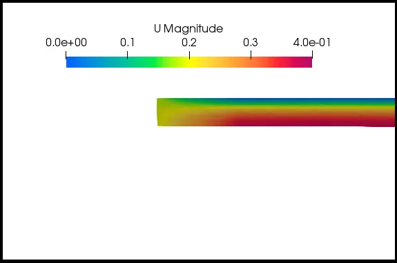
Flow before development zone close to the inlet
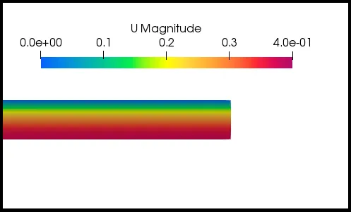
Developed flow profile at the outlet
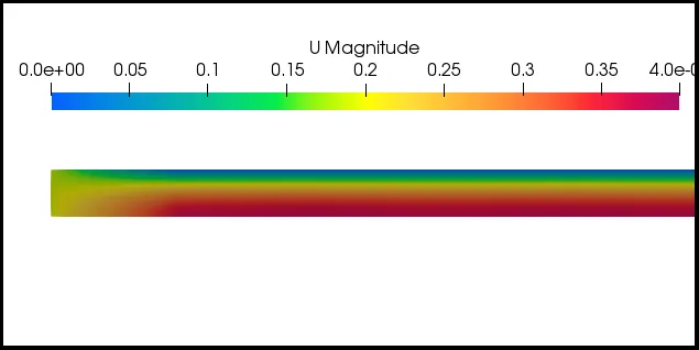
The development of the flow along the length of the pipe
Validation Hydro-dynamic length with the numerical result
The hydrodynamic length equation is given as:
`L_h = 0.06*D*R_e = 1.26 m`
From the below plot of velocity along the radius of the pipe, it is evident when multiple plots are generated at different locations from the inlet namely at distances of 0.005m, 0.0075m, 0.01m, 1.26m, 2.0m, and 2.5m a fully developed zone of the flow profile is reached at 1.26m as there exists significantly no change in the profile after this point along the length of the pipe.
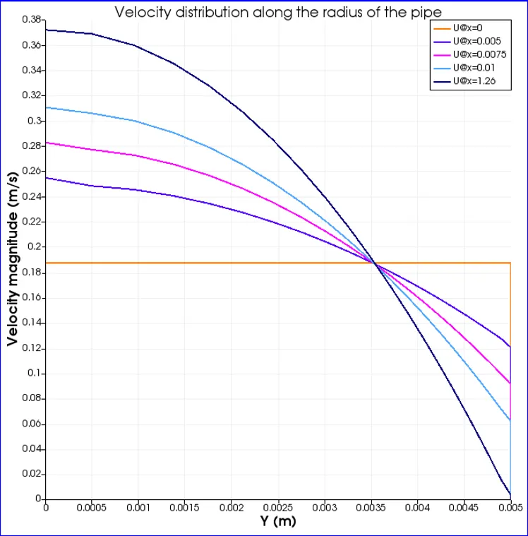
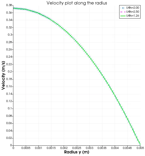
From the above plots, the flow development as moving away from the inlet is clearly visible starting from a constant velocity at the inlet due to the inlet boundary condition being defined as a constant uniform value up until the parabolic flow profile at the outlet which is due to zeroGradient boundary condition that is defined at the outlet that takes up the value numerically exact to the cells close to the outlet.
Validate the fully developed flow velocity profile with its analytical profile:
The analytical flow profile is obtained by writing a code in MATLAB that takes the inputs of flow parameters and gives the analytical value of the velocity at each location along the radius of the pipe, this can then be plotted along with the extracted data value points from the numerical result obtained from OpenFoam using ParaView post-processing tool.
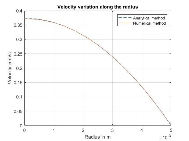
The numerically obtained value follows the analytically calculated value very closely and only a small error exists close to the centre of the pipe where the velocity is at its maximum.
Validate maximum velocity and pressure drop for fully developed flow
Maximum velocity from the numerical data is = 0.3721 m/s
Maximum velocity from the analytical calculation is = 0.3738 m/s
Which gives an error percentage of = 0.4%
The following plot provides the pressure drop variation along the length of the pipe, for which a code is written in MATLAB that takes the inputs of flow parameters and gives the analytical value of the pressure variation at each location along the length of the pipe, this can then be plotted along with the extracted data value points from the numerical result obtained from OpenFoam using ParaView post-processing tool.
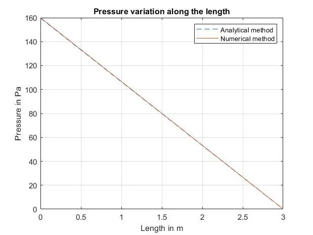
Here too, the numerically obtained value follows the analytically calculated value very closely with no significant observable error. The pressure is maximum at the inlet and drops along the length which justifies the flow direction as the fluid is transported solely due to the pressure drop along the length of the pipe.
Post-process Shear stress and validate wall shear stress for fully developed flow
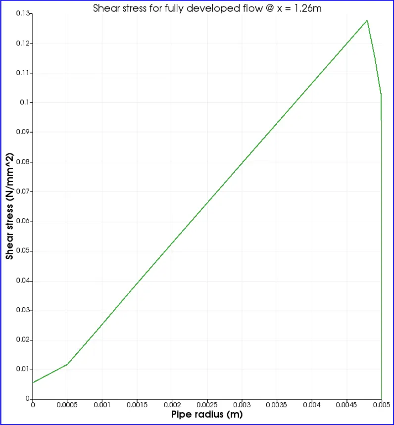
The plot provides the shear stress with respect to the distance from the wall given by the radius that is applied by the fluid flow along the length of the pipe. The wall shear can be analytically calculated by using
Darcy friction factor: `f = 64/(R_e)`
`tau_w = f/4.(rhoU_(avg)^2)/2 = 0.133 N/m^2`
which then calculated from MATLAB at every point along the radius gives a wall shear value of `0.133N/m^2` and the numerically obtained value is equal to `0.13 N/m^2`, hence the error can be calculated to be 2.2%.
This is quite acceptable for a numerical method and hence the parameters have been validated.