Week 7 - Simulation of a 1D Super-sonic nozzle flow simulation using Macormack Method
AIM: To simulate the 1D supersonic nozzle flow through a convergent-divergent nozzle using the Macormack method.
THEORY:
A convergent-divergent nozzle is a type of nozzle that is used to generate supersonic flow speed conditions from the subsonic inlet conditions. This occurs as a phenomenon of the convergent portion of the nozzle where the area decreases and the mass flow rate keeping constant the air is compressed and reaches the throat of the nozzle. Here this throat creates a shockwave effect due to which the Mach number reaches values close to 1. In the divergent portion i.e. as soon as there is a jump in Mach number from values < 1 to values >1 the behaviour of the compressibility of air changes and as it moves across the divergent section i.e. as the Area increases the speed increases and the supersonic region is achieved.
Some of the primitive variables that can be defined in order to understand this phenomenon of the convergent-divergent nozzle flow are as follows:
`x` = location or distance
`t` = time
`P` = pressure
`T` = temperature
`rho` = density
`V` = velocity
`A` = area
`M` = Mach number
Those variables with a subscript `0` are the values at the location before the convergent section, superscript with `*` are the values at the convergent throat and subscript with `e` are the values after the divergent section.
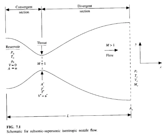
source: Computational Fluid Dynamics by JD Anderson
One such scenario will be solved in this current problem with available data and equations from the book- Computational Fluid Dynamics by JD Anderson.
Mathematical formulation:
Governing equations for Quasi 1D Supersonic nozzle flow:
The following set of equations define the phenomenon of quasi 1D supersonic nozzle flow and solving this set of equations for the primitive variables as defined previously, these variables helps capture and understand the effect of the supersonic nozzle flow.
Non-conservative form:
Continuity equation:
`(delrho)/(delt) = -rho(delV)/(delx)-rhoV(del(lnA))/(delx)-V(delrho)/(delx)`
Momentum equation:
`(delV)/(delt) = -V.(delV)/(delx)-1/gamma((delT)/(delx) + T/rho(delrho)/(delx))`
Energy equation:
`(delT)/(delt) = -V(delT)/(delx)-(gamma-1)T((delV)/(delx)+V(del(lnA))/(delx))`
Conservative form:
Continuity equation:
`(del(rhoA))/(delt)+(del(rhoAV))/(delx) = 0`
Momentum equation:
`(del(rhoAV))/(delt)+(del(rhoAV^2+(1/gamma)rhoA))/(delx)=1/gammap(delA)/(delx)`
Energy equation:
`(del(rho(e/(gamma-1)+gamma/2V^2)A))/(delt)+(del(rho(e/(gamma-1)+gamma/2V^2)VA+pAV))/(delx)=0`
Method followed:
The above-mentioned set of equations can be solved numerically with the help of a method named the Maccormack method. This method is predominantly used for solving quasi 1D supersonic nozzle flow equations. This technique is widely employed for solving hyperbolic spatial differential equations numerically, as it helps in providing a second-order accurate solution for space and time discretized variables, as observed in the current problem.
Maccormack method for Non-conservative form:
`v_(i,j)^(t+Deltat)=v_(i,j)^t+((delv)/(delt))_(avg)Deltat`
`((delv)/(delt))_(avg)=0.5[((delv)/(delt))_p+((delv)/(delt))_c]`
This method uses 2 steps to solve the variables in the discretized domain and these are the predicted and the corrector step. The solution for the gradients and rates obtained in these two steps are averaged to obtain the final solution for the time and spatial derivatives.
Predictor step:
In this step the spatial derivatives are set up as forward differences, for one primitive variable it is as described below:
`((delv)/(delt))=((delrho)/(delx))`
`((delv)/(delt))_p=((rho_(i+1,j)^t-rho_(i,j)^t)/(Deltax)+(rho_(i,j+1)^t-rho_(i,j)^t)/(Deltay))`
Once the spatial derivative is evaluated, its time derivative can be evaluated as described below with the predicted spatial derivative:
`v_(i,j)^(t+Deltat)=v_(i,j)^t+((delv)/(delt))_pDeltat`
Corrector step:
In the corrector step, the derivative is evaluated as a backward difference, for which the values are obtained from the predictor step.
`((delv)/(delt))_c= ((rho_(i,j)^(t+Deltat)-rho_(i-1,j)^(t+Deltat))/(Deltax)+(rho_(i,j)^(t+Deltat)-rho_(i,j-1)^(t+Deltat))/(Deltay))`
Time step evaluation:
The time step for which the simulation will be run is evaluated with the help of the Courant number which is kept equal to 0.5, `Co = 0.5`
`Deltat=Co(Deltax)/(V+a)`
Maccormack method for Conservative form:
The method followed involves the same steps but the variables to be evaluated in solving the conservative form of equations are different, for which the code is written for the following form of solution equations:
`U_1=rhoA`
`U_2=rhoAV`
`U_3=rho(e/(gamma-1)+gamma/2V^2)A`
`F_1=rhoAV`
`F_2=rhoAV^2+(pA)/(gamma)`
`F_3=rho(e/(gamma-1)+(gamma)/2V^2)VA+pAV`
`J_2=1/gammap(delA)/(delx)`
Predictor step:
In this step the spatial derivatives are set up as forward differences, for one primitive variable it is as described below:
`((delU_1)/(delt))_i^t=-((F_1)_(i+1)-(F_1)_i)/(Deltax)`
`(U_1)_i^(t+Deltat) = (U_1)_i^t + ((delU_1)/(delt))_i^tDeltat`
These can be used for the calculation of primitive variables such as `rho` and `T`
Corrector step:
In the corrector step, the derivative is evaluated as a backward difference, for which the values are obtained from the predictor step.
`((delU_1)/(delt))_i^t=-((F_1)_i-(F_1)_(i-1))/(Deltax)`
`((delU)/(delt))_(avg) = 0.5[((delU_1)/(delt))_i^t+((delU_1)/(delt))_i^(t+Deltat)]`
`(U_1)_i^(t+Deltat) = (U_1)_i^t + ((delU_1)/(delt))_(avg)Deltat`
Finally with the corrected values the primitive variables can be evaluated using:
`rho = (U_1)/(A)`
`V = U_2/U_1`
`T=(gamma-1)((U_3)/(U_1)-gamma/2V^2)`
Boundary conditions applied:
`A = 1+2.2(x-1.5)^2` `0<=x<=3`
Non-conservative form:
Initial conditions at t=0:
`rho=1-0.3146x`
`T=1-0.2314x`
`V=(0.1+1.09x)T^(1/2)`
Inlet BC:
`V_1=2V_2-V_3`
Outlet BC:
`V_N=2V_(N-1)-V_(N-2)`
`rho_N=2rho_(N-1)-rho_(N-2)`
`T_N=2T_(N-1)-T_(N-2)`
Conservative form:
Initial conditions:`U_3=U_1(T/(gamma-1)+gamma/2V^2)`
for `0<=x<=0.5`
`rho=1.0`
`T=1.0`
for `0.5<=x<=1.5`
`rho=1.0-0.366(x-0.5)`
`T=1.0-0.167(x-0.5)`
for `1.5<=x<=3.5`
`rho=0.634-0.3879(x-1.5)`
`T=0.833-0.3507(x-1.5)`
`V=U_2/(rhoA)=0.59/(rhoA)`
Inlet BC:
`U_(1(i=1)) =(rhoA)_(i=1)=A_(i=1)`
`U_(2(i=1))=2U_(2(i=2))-U_(2(i=3))`
`U_3=U_1(T/(gamma-1)+gamma/2V^2)`
Outlet BC:
`(U_1)_N=2(U_1)_(N-1)-(U_1)_(N-2)`
`(U_2)_N=2(U_2)_(N-1)-(U_2)_(N-2)`
`(U_3)_N=2(U_3)_(N-1)-(U_3)_(N-2)`
CODE:
Main program:
This program creates a mesh and sets the time steps for the simulation. Functions for solving the quasi 1D supersonic nozzle flow case using both conservative and non-conservative approaches are called and the results for the primitive variables and their values at the throat are then obtained and plotted in the final section of the program. The variation of primitive variables along the throat and the variation of primitive variables at the throat with respect to time are plotted as a comparison of the conservative and the non-conservative forms of the equation.
clear all
close all
clc

% time and space descritization
n = 51;      % number of grid points
nt = 1400;   % number of time steps
cfl = 0.5;   % CFL number for convergence time step calculation

% v - velocity, v_T - velocity at throat
% rho - density, rho_T - density at throat
% T - temperature, T_T - temperature at throat
% m - mass, m_T - mass at throat
% v - Mach number, M_T - Mach number at throat
% p - pressure, p_T - pressure at throat

% function for solving the conservative form
tic;
[x1,v1,rho1,T1,m1,M1,p1,v_T1,rho_T1,T_T1,m_T1,M_T1,p_T1] = conservative(n,nt,cfl);
simulation_time_C = toc;

% function for solving the non-conservative form
tic;
[x2,v2,rho2,T2,m2,M2,p2,v_T2,rho_T2,T_T2,m_T2,M_T2,p_T2] = non_conservative(n,nt,cfl);
simulation_time_NC = toc;

% plots for Conservative form

% plot for density
figure(5)
subplot(4,1,1)
plot(x1,rho1)
hold on
plot(x2,rho2,'*')
title(sprintf('Variation of the primitive variables along the nozzle (Timesteps = %d)',nt));
xlabel('Length')
ylabel('Density')
legend('Conservative','Non-conservative')

% plot for temperature
subplot(4,1,2)
plot(x1,T1)
hold on
plot(x2,T2,'*')
xlabel('Length')
ylabel('Pressure')
legend('Conservative','Non-conservative')

% plot for Mach number
subplot(4,1,3)
plot(x1,M1)
hold on
plot(x2,M2,'*')
xlabel('Length')
ylabel('Mach number')
legend('Conservative','Non-conservative')

% plot for pressure
subplot(4,1,4)
plot(x1,p1)
hold on
plot(x2,p2,'*')
xlabel('Length')
ylabel('Pressure')
legend('Conservative','Non-conservative')

% Time variation of primitive variables at throat
time = (1:nt);

figure(6)
subplot(4,1,1)
plot(time,rho_T1,'r')
hold on
plot(time,rho_T2,'b')
title(sprintf('Time-wise variation of the primitive variables at throat'));
xlabel('Time steps')
ylabel('Density')
legend('Conservative','Non-conservative')

% plot for temperature
subplot(4,1,2)
plot(time,T_T1,'r')
hold on
plot(time,T_T2,'b')
xlabel('Time steps')
ylabel('Temperature')
legend('Conservative','Non-conservative')

% plot for Mach number
subplot(4,1,3)
plot(time,M_T1,'r')
hold on
plot(time,M_T2,'b')
xlabel('Time steps')
ylabel('Mach number')
legend('Conservative','Non-conservative')

% plot for pressure
subplot(4,1,4)
plot(time,p_T1,'r')
hold on
plot(time,p_T2,'b')
xlabel('Time steps')
ylabel('Pressure')
legend('Conservative','Non-conservative')
Function for conservative form:
This function evaluates the primitive variables at the points along the length of the nozzle for which the discretization was done and solves the conservative form of the equation and returns the values for the primitive variables and the variables at the throat as vectors to the main program. The final section also plots the variation of mass flow rate with respect to different time steps and the residual values for the iterations performed.
function [x,v,rho,T,m,M,p,v_T,rho_T,T_T,m_T,M_T,p_T] = conservative(n,nt,cfl)

% inputs
x = linspace(0,3,n);
dx = x(2) - x(1);
gamma = 1.4;

% initial conditions

% area
a = 1+2.2*(x-1.5).^2;

rho = ones(1,n);
T = ones(1,n);

% initial profile
% loop for setting density and temperature
for node = 1:n
    if (x(node)<=0.5)
        rho(node) = 1;
        T(node) = 1;
    elseif (x(node)>0.5 && x(node)<=1.5)
        rho(node) = 1-0.366*(x(node)-0.5);
        T(node) = 1-0.167*(x(node)-0.5);
    else
        rho(node) = 0.634-0.3879*(x(node)-1.5);
        T(node) = 0.833-0.3507*(x(node)-1.5);
    end
end

  % depends on the number of grid points n

% velocity
v = 0.59./(rho.*a);

% solution term
p = rho.*T;
U1 = rho.*a;
U2 = rho.*a.*v;
U3 = U1.*((T/(gamma-1))+(0.5*gamma*v.^2));

% Time step size calculation from Courant number
dt = min(cfl.*(dx./((sqrt(T))+v)));

% Outer time loop
for t = 1:nt

    % copies
    U1_old = U1;
    U2_old = U2;
    U3_old = U3;

    %flux vector
    F1 = U2;
    F2 = ((U2.^2)./U1)+((gamma-1)/gamma)*(U3-((gamma/2)*((U2.^2)./U1)));
    F3 = ((gamma*U2.*U3)./U1)-(((gamma*(gamma-1))/2)*((U2.^3)./(U1.^U2)));

    % Predictor method
    for j = 2:n-1

        dF1dx(j) = (F1(j+1)-F1(j))/dx;
        dF2dx(j) = (F2(j+1)-F2(j))/dx;
        dF3dx(j) = (F3(j+1)-F3(j))/dx;
        dloga_dx(j) = (log(a(j+1))-log(a(j)))/dx;
        dadx(j) = (a(j+1)-a(j))/dx;
        J(j) = (1/gamma)*rho(j)*T(j)*dadx(j);

        % continuity equation
        dU1dt_p(j) = -dF1dx(j);

        % momentum equation
        dU2dt_p(j) = -dF2dx(j) + J(j);

        % energy equation
        dU3dt_p(j) = -dF3dx(j);

        % Solution update
        U1(j) = U1(j) + dU1dt_p(j)*dt;
        U2(j) = U2(j) + dU2dt_p(j)*dt;
        U3(j) = U3(j) + dU3dt_p(j)*dt;
    end

    % primitive variables
    rho = U1./a;
    v = U2./U1;
    T = (gamma-1)*((U3./U1)-((gamma*v.^2)/2));

    % updating the flux terms
    F1 = U2;
    F2 = ((U2.^2)./U1) + (((gamma-1)/gamma)*(U3-(gamma*U2.^2)./(2*U1)));
    F3 = ((gamma*U2.*U3)./U1)-((gamma*(gamma-1)/2)*((U2.^3)./(U1.^U2)));


    % Corrector step
    for k = 2:n-1

        dF1dx(k) = (F1(k)-F1(k-1))/dx;
        dF2dx(k) = (F2(k)-F2(k-1))/dx;
        dF3dx(k) = (F3(k)-F3(k-1))/dx;
        dloga_dx(k) = (log(a(k))-log(a(k-1)))/dx;

        dadx(k) = (a(k)-a(k-1))/dx;
        J(k) = (1/gamma)*rho(k)*T(k)*dadx(k);

        % continuity equation
        dU1dt_c(k) = -dF1dx(k);

        % momentum equation
        dU2dt_c(k) = -dF2dx(k) + J(k);

        % energy equation
        dU3dt_c(k) = -dF3dx(k);

    end

    % compute the average time derivative

    dU1dt = 0.5*(dU1dt_p + dU1dt_c);
    dU2dt = 0.5*(dU2dt_p + dU2dt_c);
    dU3dt = 0.5*(dU3dt_p + dU3dt_c);

    % Final solution update

    for i = 2:n-1

        U1(i) = U1_old(i) + dU1dt(i)*dt;
        U2(i) = U2_old(i) + dU2dt(i)*dt;
        U3(i) = U3_old(i) + dU3dt(i)*dt;

    end

    % Apply the boundary consitions
    % Inlet BC
    U1(1) = rho(1)*a(1);
    U2(1) = 2*U2(2)-U2(3);
    v(1) = U2(1)/U1(1);
    U3(1) = U1(1)*((T(1)/(gamma-1))+(0.5*gamma*v(1)^2));

    % Outlet BC
    U1(n) = 2*U1(n-1)-U1(n-2);
    U2(n) = 2*U2(n-1)-U2(n-2);
    U3(n) = 2*U3(n-1)-U3(n-2);

    % primitive variables
    rho = U1./a;
    v = U2./U1;
    T = (gamma-1)*((U3./U1)-(gamma/2)*(v.^2));

    % mass
    m = rho.*a.*v;
    % mach number
    M = v./((T).^0.5);
    % pressure
    p = rho.*T;

    % values of the primitive variables inside the throat
    throat = index_function(a,1); % external function to compute the index at which area = 1

    rho_T(t) = rho(throat);
    v_T(t) = v(throat);
    T_T(t) = T(throat);
    m_T(t) = m(throat);
    p_T(t) = p(throat);
    M_T(t) = M(throat);

    % residues at throat
    U1_res(t) = dU1dt(throat);
    U2_res(t) = dU2dt(throat);
    U3_res(t) = dU3dt(throat);

    % Variation of Mass flow rate distribution inside the nozzle at different time steps

    figure(1)
    if t == 100
        plot(x, m, 'r')
        hold on
    elseif t == 200
        plot(x, m, 'b')
        hold on
    elseif t == 500
        plot(x, m, 'g')
        hold on
    elseif t == 1000
        plot(x, m, 'k')
        hold on
    elseif t == 1400
        plot(x, m, 'y')
        xlabel('Length')
        ylabel('Mass flow rate distribution')
        title('Mass flow rate for Conservative approach at different time steps')
        legend('100 time steps','200 time steps','500 time steps','1000 time steps','1400 time steps')
    end
end

time_vector = linspace(1,nt,nt);

figure(2)
plot(time_vector,U1_res,'r');
hold on
plot(time_vector,U2_res,'b')
hold on
plot(time_vector,U3_res,'g')
xlabel('Residual values')
ylabel('Time steps')
legend('U1','U2','U3')
title('Residual plot for Conservative approach')

end
Function for non-conservative form:
This function evaluates the primitive variables at the points along the length of the nozzle for which the discretization was done and solves the non-conservative form of the equation and returns the values for the primitive variables and the variables at the throat as vectors to the main program. The final section also plots the variation of mass flow rate with respect to different time steps and the residual values for the iterations performed.
function [x,v,rho,T,m,M,p,v_T,rho_T,T_T,m_T,M_T,p_T] = non_conservative(n,nt,cfl)

% inputs
x = linspace(0,3,n);
dx = x(2) - x(1);
gamma = 1.4;

% initial profile
rho = 1-0.3146*x;  % density
T = 1-0.2314*x;    % temperature
v = (0.1+1.09*x).*T.^0.5;  % velocity

% area
a = 1+2.2*(x-1.5).^2;   % depends on the number of grid points n

% Time step size calculation from Courant number
dt = min(cfl.*(dx./((sqrt(T))+v)));

% Outer time loop
for t = 1:nt
    rho_old = rho;
    v_old = v;
    T_old = T;

    % Predictor method
    for j = 2:n-1
        % predictor time derivative for density

        dvdx = (v(j+1)-v(j))/dx; % velocity derivative
        drhodx = (rho(j+1)-rho(j))/dx; % density derivative
        dTdx = (T(j+1)-T(j))/dx; % temperature derivative
        dloga_dx = (log(a(j+1))-log(a(j)))/dx; % area derivative

        % Continuity equation
        drhodt_p(j) = -rho(j)*dvdx -rho(j)*v(j)*dloga_dx -v(j)*drhodx;

        % Momentum equation
        dvdt_p(j) = -v(j)*dvdx -(1/gamma)*(dTdx + (T(j)/rho(j))*drhodx);

        % Energy equation
        dTdt_p(j) = -v(j)*dTdx -(gamma-1)*T(j)*(dvdx + v(j)*dloga_dx);

        % Solution update
        rho(j) = rho(j) + drhodt_p(j)*dt;
        v(j) = v(j) + dvdt_p(j)*dt;
        T(j) = T(j) + dTdt_p(j)*dt;
    end


    % Corrector step
    for j = 2:n-1
        % predictor time derivative for density

        dvdx = (v(j)-v(j-1))/dx; % velocity derivative
        drhodx = (rho(j)-rho(j-1))/dx; % density derivative
        dTdx = (T(j)-T(j-1))/dx; % temperature derivative
        dloga_dx = (log(a(j))-log(a(j-1)))/dx; % area derivative

        % Continuity equation
        drhodt_c(j) = -rho(j)*dvdx -rho(j)*v(j)*dloga_dx -v(j)*drhodx;

        % Momentum equation
        dvdt_c(j) = -v(j)*dvdx -(1/gamma)*(dTdx + (T(j)/rho(j))*drhodx);

        % Energy equation
        dTdt_c(j) = -v(j)*dTdx -(gamma-1)*T(j)*(dvdx + v(j)*dloga_dx);

    end

    % compute the average time derivative

    drhodt = 0.5*(drhodt_p + drhodt_c);
    dvdt = 0.5*(dvdt_p + dvdt_c);
    dTdt = 0.5*(dTdt_p + dTdt_c);

    % Final solution update

    for i = 2:n-1

        rho(i) = rho_old(i) + drhodt(i)*dt;
        v(i) = v_old(i) + dvdt(i)*dt;
        T(i) = T_old(i) + dTdt(i)*dt;

    end

    % Apply the boundary consitions
    % Inlet BC
    v(1) = 2*v(2) - v(3);

    % Outlet BC
    v(n) = 2*v(n-1) - v(n-2);
    rho(n) = 2*rho(n-1) - rho(n-2);
    T(n) = 2*T(n-1) - T(n-2);

    % primitive variables

    % mass
    m = rho.*a.*v;
    % mach number
    M = v./((T).^0.5);
    % pressure
    p = rho.*T;

    % values of the primitive variables inside the throat
    throat = index_function(a,1); % external function to compute the index at which area = 1
    rho_T(t) = rho(throat);
    v_T(t) = v(throat);
    T_T(t) = T(throat);
    m_T(t) = m(throat);
    p_T(t) = p(throat);
    M_T(t) = M(throat);

    % residues at throat
    v_res(t) = dvdt(throat);
    rho_res(t) = drhodt(throat);
    T_res(t) = dTdt(throat);

    % Variation of Mass flow rate distribution inside the nozzle at different time steps

    figure(3)
    if t == 100
        plot(x, m, 'r')
        hold on
    elseif t == 200
        plot(x, m, 'b')
        hold on
    elseif t == 500
        plot(x, m, 'g')
        hold on
    elseif t == 1000
        plot(x, m, 'k')
        hold on
    elseif t == 1400
        plot(x, m, 'y')
        xlabel('Length')
        ylabel('Mass flow rate distribution')
        title('Mass flow rate for Non-conservative approach at different time steps')
        legend('100 time steps','200 time steps','500 time steps','1000 time steps','1400 time steps')
    end

end

time_vector = linspace(1,nt,nt);

figure(4)
plot(time_vector,v_res,'r');
hold on
plot(time_vector,rho_res,'b')
hold on
plot(time_vector,T_res,'g')
xlabel('Residual values')
ylabel('Time steps')
legend('Velocity','Density','Temperature')
title('Residual plot for Non-conservative')

end
Function for indexing:
An external function for indexing was written that is called by the conservative and no-conservative functions in order to locate the index of the element in the primitive variables' array that exactly determines the position of the throat which is at the location where the Area of the throat is 1.
function index = index_function(x,x_value)

    for i=1:length(x)
        if x(i) == x_value
            index = i;
        end
    end

end
Results:
Figure1: Steady-state distribution of primitive variables inside the nozzle
This figure plots the variation of primitive variables inside the nozzle along the length of the nozzle for the conservative and non-conservative forms of the governing equations and a slight variation is observed at the region close to the end of the nozzle.
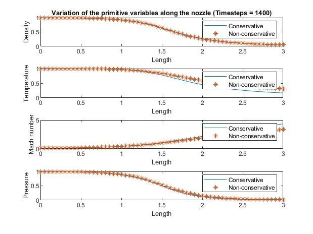
Figure 2: Time-wise variation of the primitive variables
The following plot provides the time-wise variation of the primitive variables for conservative and non-conservative forms of the governing equations. It is clear that after 600-800 time steps the values converge and not much variation further on up to 1400 time steps. There are considerably high initial variations in the Non-conservative approach compared to the conservative approach.
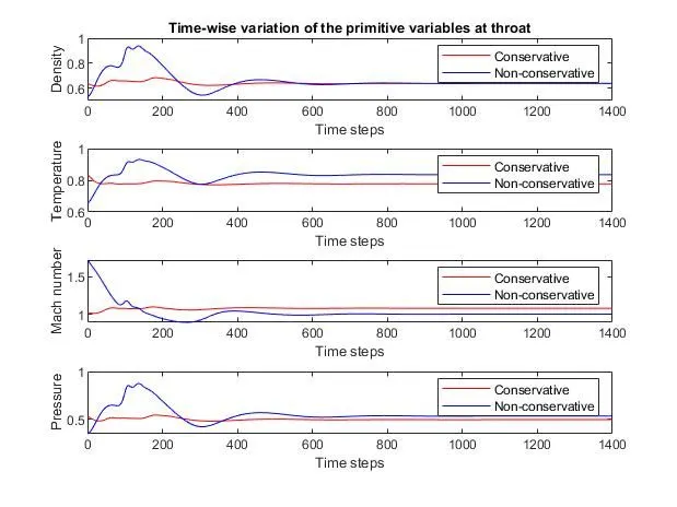
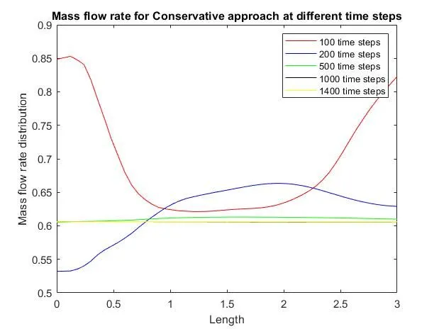
Figure 3: Variation of Mass flow rate distribution inside the nozzle at different time steps during the time-marching process
This figure shows the variation of Mass flow rate distribution inside the nozzle at different time steps during the time-marching process for a conservative approach, as observable from the plot it is clear that after 500 time steps the solution is almost constant for both 1000 and 1400 time steps indicating constant mass flow rate which confirms continuity for the problem.
This figure shows the variation of Mass flow rate distribution inside the nozzle at different time steps during the time-marching process for a non-conservative approach, as observable from the plot it is clear that after 500 time steps the solution is almost constant for both 1000 and 1400 time steps indicating constant mass flow rate which confirms continuity for the problem.
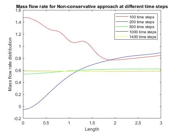
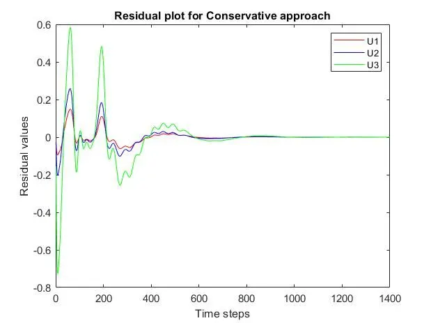
Figure 4: Residuals plot
The following plot shows the variation of the residuals for the variables evaluated in the conservative approach and it is observable that after 800 time steps the values reach close to 0and it is constant up to 1400 time steps which is the end of the simulation.
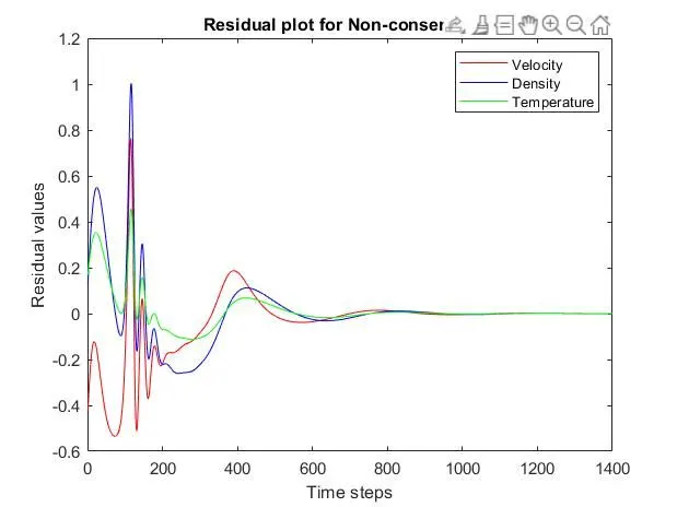
The following plot shows the variation of the residuals for the variables evaluated in the non-conservative approach and it is observable that after 800 time steps the values reach close to 0and it is constant up to 1400 time steps which is the end of the simulation.
Grid indipendence test:
|
Primitive variables at the throat |
n=31 Conservative |
n=31 Non-conservative |
n=51 Conservative |
n=51 Non-conservative |
n=71 Conservative |
n=71 Non-conservative |
| Density | 0.6533 | 0.6387 | 0.6367 | 0.6367 | 0.6373 | 0.6366 |
| Temperature | 0.7885 | 0.8365 | 0.7778 | 0.8335 | 0.7788 | 0.8348 |
| Mach number | 1.0485 | 0.9994 | 1.0795 | 0.9998 | 1.0762 | 1.0000 |
| Pressure | 0.5152 | 0.5342 | 0.4952 | 0.5327 | 0.4963 | 0.5314 |
From the grid independence test with reference to the primitive variables at the throat, it is clear that the difference of values between the solutions for when the number of grid points is set to 51 and 71 is not significant and hence 51 grid points scenario can be and is used for the further simulation study.