Week 9 - FVM Literature Review

What is Finite Volume Method(FVM) ?

• For Fluid flow, heat & mass transfer problems the more important governing guiding princple is the 'principle of conservation'.
• When we dervided the conservation form of Governing equations in Intergral form over an arbitary CV & when it is extended to non-overlapping a set of CV & our conservation laws are valid at each of this CV, using this feature we can come up with a discretization method to solve problems. By this way can overcome the limitations of FDM.
• It is one of the discretization method used to solve PDE'S numerically that represent the conervation laws. -mass,momentum & energy. Here in FVM, it is most common that PDE's Gov.Eqns. are used to derive back to integral over finite volume.
• The descritised algebraic equations are fluxes based consevative and adhere to boundedness & transportiveness properties.So,this numerical results will only be physically realistic.
• It is widely used method in CFD tools & comercial solver packages like Open Foam,CFD etc.

Major differences between FDM & FVM ?

FDM

• It is the oldest & simplest method.
• In FDM the derivaties of gov.eqns. are expressed in the form algebraic equations using Taylor series expansion with appropriate truncation.
• Here, we divide the domian into discrete grid points all over or represent the whole domain by collection of grid points and Gove.eqns are solved for all these grid points.
• The Resulting system of equation doesn't involve any conservativeness or fluxes of variable.
• FDM is limited to (cartesian) structured grid & when complex goemetries are inlvoved,variable transformation is used with mapping functions, which is being tidious & some times impossible.

FVM

• Implemented method for some drawbacks of FDM & bit more expensive in formulation.
• In FVM the valid governing PDE are intergrated over finite control volume(or cell) & by applying Gauss-divergence theorem and aproximating to average values to cell & face centre a descritised equations are obtained.
• Here, we divide the domain into no. of subdomains (defined by grid points) called finite control volume of any arbitary shape and Gove.eqns are solved for all these CV.
• The Resulting system of equation involve any conservativeness or fluxes of variable.
• FVM can accomodate any type of grid and hence it is naturally suitable for complex goemtries.

Steps in FV solution :-

Consider an 1D steady state diffusion linear heat conduction equation as an example

gov.eqn - `(del)/(delx)(alpha*(delT)/(delx)) +S =0`

where, alpha = Thermal diffusitivity or diffusion coeffient

S = source term.

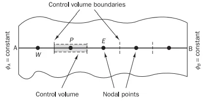
1) Grid generation

In above the domain is divided into 5-CV & a system of notation is established in below way, here for analysis main cell centroid denoted by 'P' & its neighbours as West & East and faces at small w&e.

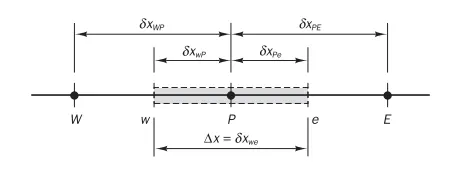
Note : There are two approaches of grid

1. face centred approach - used on structred grid & computational nodes are defined in such way that CV faces lie midway b/w the faces.
2. cell centred approach - used on Unstructred grid & computational nodes are at centre of CV.

2) Discretisation

The key step of FVM isto integrate the gov.eqn. in PDE form over the CV.

`int_V(del)/(delx)(alpha*(delT)/(delx)) dV+int_VSdV = 0`

Now converting diffusion flux term from volume integral into surface integral using Guass-divergnece theorem

`int_salpha*(delT)/(delx) dvecS+int_VSdV = 0`

Assuming flux(T) varies lineraly over the faces & can be represented by its value at face centre and also source term to its mean value at cell centre. This approximation will give 2nd order accuracy.

Also, assuming gradient dT/dx at face centres & alpha varying ingeneral.

surface vector is equal to product of face area and unit vector. Here surface vector at west is pointing outwards (-ve x direction).

`(alpha*A*(delT)/(delx) )_e- (alpha*A*(delT)/(delx) )_w+barSdeltaV = 0`

It is an very attractive feature of the finite volume method that the discretised
equation has a clear physical interpretation, where diffusive flux of T leaving the east face minus the diffusive flux of T entering
the west face is equal to the generation of T, i.e. it constitutes a balance equation for T over the control volume.

In order to derive useful forms of the discretised equations, the interface values of the gradient flux (T) and the diffusion coefficient(alpha) are defined and evaluated, assuming linear approximation.

`alpha_w = (alpha_W +alpha_P)/2`

`alpha_e = (alpha_E+alpha_P)/2`

`((delT)/(delx) )_e= (T_E - T_P)/(deltax_(PE))`

`((delT)/(delx) )_w= (T_P - T_W)/(deltax_(PW))`

the source term S may be a function of the dependent variable, then approximates to linear form

`barSdeltaV = S_u +S_p*T_p`

Substituting & Re-arranging we get

`(alpha_e/(deltax_(PE))*A_e + alpha_w/(deltax_(WP))*A_w - S_p)T_P = (alpha_w/(deltax_(WP))*A_w )T_W +(alpha_e/(deltax_(PE))*A_e)T_E+S_u`

The co-efficients of T can be represented as 'a', then

`a_PT_p =a_WT_W +a_ET_E+S_u`

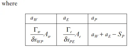
3) Solution of equations

Discretised equations of above last form must be set up at each of the nodal points in order to solve a problem. For control volumes that are adjacent to the domain boundaries the general discretised equation (4.11) is modified to incorporate boundary conditions. The resulting system of linear algebraic equations is then solved to obtain the distribution of the property T at nodal points.

Interpolation schemes/discretization schemes in FVM ?

Let us consider below setup for understanding the different types of schemes

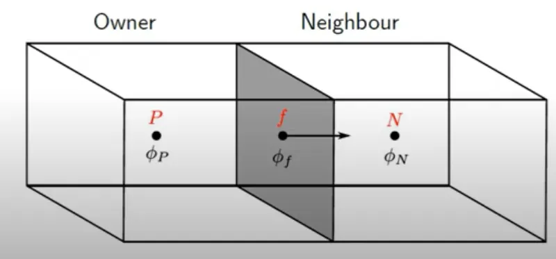
Here, 2 CV named owner (main cell) & neighbour,with cenrtroids noted in figure. Also, consider the `phi`as any flow quantity (T,p,U)

In FVM the values are stored at cell centres and with this will approxiamte face centre values using below face Interpolation schemes :-

1)Linear/central differencing :

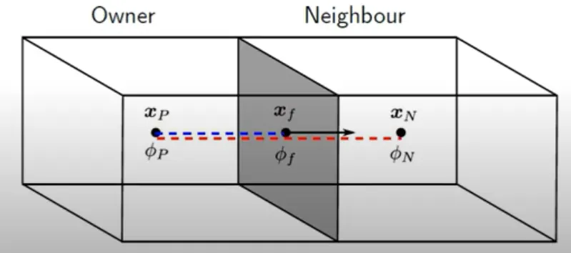
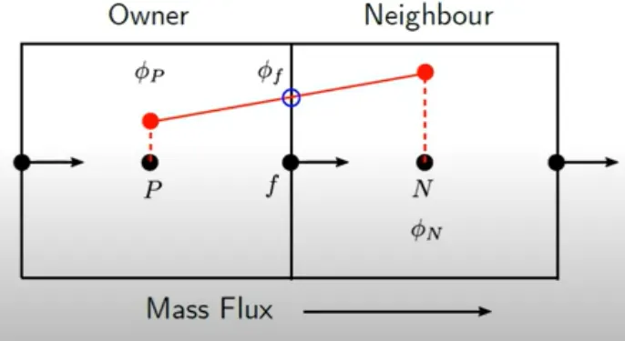
Linear diffenencing is basically straight foward / linear interpolation scheme and it is termed as second order accurate.

The value at face centre is given by

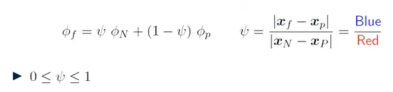
the value of `psi`varies depending on the structure of cells over the entire CV. When distance b/w nodal points are equal then it will be average of both.

This scheme is Unbounded & prone to obtain oscillations in solution. CDS can be used for diffusion terms & should not be used for convection term in RANS N.S.Eqn. solver.

2)Upwind differncing scheme :

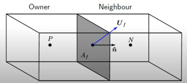
Upwind differncing depends on the direction of mass flux, it provides the importanat info. of direction mass flow rate. given below

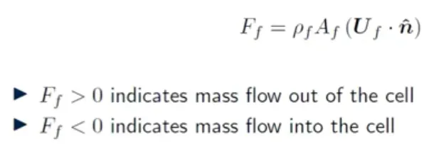
With info. of flow direction we are assuming the same nodal value as face value at the centre. Hence, this first order accurate & has no variation across the cell faces and it is constnat b/w cell centroid & cell face.

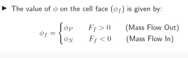
Upwind schemes tend to smear-out (loss of resolution) the solution and not accurate. However, they are the most stable scheme for convection dominated flows , in which they are used to get the Intial solution for some circumstences where convection terms is diverging, bad mesh or simulation going unsteady and then later switch to other accurate schemes get required final solution.

3) Linear upwind/hybrid differnecing scheme -

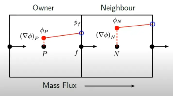
This scheme is very popular and most used in CFD codes, even here the face value is dependent on the mass flux direction.

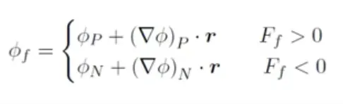
But, here the accuracy is improved by adding gradient of flow quatities at cell centroid with dot product of vector(r) b/w cell centroid & face.This is second order accurate because it linearly varies b/w cell centroid & face. Even, this is popularly used for convection terms with increase in accuracy after upwind differencing.

However,this may go unstable and can be observed from below figure

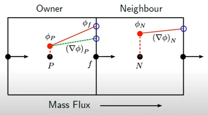
If face value quantity being projected by the gradient is too steep, as indicated by the red line, where the values of interpolated face centre quantity is larger than neigbour & as well as owner cell. This isn't physical & will clearly lead to instability in simulations & eddies formation.

To overcome this we need to limit the face value within owner & neibhour cell. Done by flux limiter explanied below -

What are the Flux limiters in FVM ?

The gradient limiters reduces the gradient values of quantities at Owner & neighbour cell centroids so that extrapolated face value will not cross the actual values of quatity at Owner & neighbour cell centroids. Thus, obtaining a stable accurate solution.

The gradient multiplier is denoted by `varphi` which will control stability. This value can be varied from 0 to 1. If the value is '1' then we have not limited & if '0' it result back to upwind differencing.

Some advanced differencing schemes are :-

1)TVD schemes

2)Gama differnecing

Refrences used :

1) https://youtu.be/JVE0fNkc540

2) https://youtu.be/ksHCHF2BKes