Week 5.1 - Mid term project - Solving the steady and unsteady 2D heat conduction problem
Code written in such way that , for Steady state for every Iteration in Implicit method seperate 'if' loops include all common terms. But in Unsteady state tried to optimise by using 'If' conditions often.
As all methods & answer plots con be obtained in this single program, selection to be done accordingly.
clear all
close all
clc
% 2D Heat conduction analysis

% Defining 2D domain
% Grid points in square domain
nx= 10;
ny=10;
L =1; % Length in meter
% Grid points along x & y spatial
x= linspace(0,L,nx);
y = linspace(0,L,ny);
% Grid spacing
dx = x(2)-x(1);
dy = y(2)- y(1);

% Initialiation of tempertaure
T_in = ones(nx,ny);
T_in(:,:) = 300; % T0 = 300k (kelvin)
% Boundary conditions
T_in(:,1) = 400; %Left Boundary = 400 K
T_in(1,:) = 600; %Top Boundary = 600 K
T_in(:,end) = 800; %Right Boundary = 800 K
T_in(end,:)=900; %Bottom Boundary = 900 K

%Assuming average values at corner nodes
T_in(1,1) = (600+400)/2;
T_in(10,10) = (800+900)/2;
T_in(1,10) = (600+800)/2;
T_in(10,1) = (900+400)/2;

%guess vector for unkown temperatue
Told = T_in;
T=Told;
T_prev=T_in;

%loop counters
jacobi_iter=1;
 gs_iter =1;
 sor_iter =1;

omega = 1.15 ; %SOR Relaxation factor

% Accuracy of convergence
error = 909;
tol = 1e-4; % tolerence

% Selection of state of conduction for analysis
state = 1; % steady
% state = 2; % unteady

%Unsteady solution method selection
 method = 1; % Explicit
% method = 2; % Implicit

% Selection of 3 differenet itterative technique
iterative_solver = 1; %Jacobi
% iterative_solver = 2; %Gauss -seidel
% iterative_solver = 3; %SOR


if state == 1
% 1) Steady state conduction equation
% d^2T/dx^2 + d^2T/dy^2 = 0

%FD approximation of 2nd order PDE | Central differencing - 2nd order accuracy
% (T(i-1,j)+T(i,j)+T(i+1,j))/dx^2) + (T(j-1,i)+T(i,j)+T(j+1,i))/dy^2) =0

% Steady state implicit function
% T(i-1,j) = ((Told(i+1,j)+Told(i-1,j))/dx^2+(Told(i,j+1)+Told(i,j-1))/dy^2)/(2*(dx^2+dy^2)/(dx^2*dy^2))


% a) Jacobi technique

if iterative_solver ==1

 %Convergence loop
while (error>tol)
    %space loop
for i = 2:nx-1;
    for j=2:ny-1;
k = (2*(dx^2+dy^2)/(dx^2*dy^2));
term1 = (Told(i+1,j)+Told(i-1,j))/dx^2;
term2  = (Told(i,j+1)+Told(i,j-1))/dy^2;
T(i,j) = (term1+term2)/k;
    end
end
  error = max(max(abs(Told-T)));
    Told = T; %upadte Told
    jacobi_iter=jacobi_iter+1;

end
    contourf(x,y,T,'showtext','on')
    set(gca,'YDIR','reverse')
    xlabel('X-axis')
    ylabel('Y-axis')
    title(sprintf('Steady state heat conduction \n jacobi iteration no. = %d',jacobi_iter));

end


%Gauss-seidel technique

if iterative_solver == 2;
   %Convergence loop
while (error>tol)
      %space loop
for i = 2:nx-1;
    for j=2:ny-1;
k = (2*(dx^2+dy^2)/(dx^2*dy^2));
%Updating (i-i),(j-1) calculated new guess values
term1 = (Told(i+1,j)+T(i-1,j))/dx^2;
term2  = (Told(i,j+1)+T(i,j-1))/dy^2;
T(i,j) = (term1+term2)/k;
    end
end
  error = max(max(abs(Told-T)));
    Told = T;  %upadte Told
    gs_iter=gs_iter+1;

end
    contourf(x,y,T,'showtext','on')
    set(gca,'YDIR','reverse')
    xlabel('X-axis')
    ylabel('Y-axis')
    title(sprintf('Steady state heat conduction \n Gauss-seidel iteration no. = %d',gs_iter));
end


%Successive over-relaxation technique

if iterative_solver == 3;

while (error>tol)
for i = 2:nx-1;
    for j=2:ny-1;
k = (2*(dx^2+dy^2)/(dx^2*dy^2));
term1 = (Told(i+1,j)+T(i-1,j))/dx^2;
term2  = (Told(i,j+1)+T(i,j-1))/dy^2;
%Applying SOR for Gauss-seidel
T(i,j) = ((1-omega)*Told(i,j))+(omega*(term1+term2)/k);
    end
end
  error = max(max(abs(Told-T)));
    Told = T;  %upadte Told
    sor_iter=sor_iter+1;
end
   contourf(x,y,T,'showtext','on')
    set(gca,'YDIR','reverse')
    xlabel('X-axis')
    ylabel('Y-axis')
    title(sprintf('Steady state heat conduction \n SOR iteration no. = %d',sor_iter));
end

end

if state == 2

% 2) Unsteady/Transient state analysis equation
% d^2T/dt^2 = c*(d^2T/dx^2 + d^2T/dy^2 )

c=1.5;% Thermal diffusitivity in m/sec^2
dt = 0.0015; %Time step in sec
nt = 1500; % No. of time steps

CFL = c*dt*((1/dx^2)+(1/dy^2)); % CFL stability check <=0.5;

if (method==1) % Explicit
%FD approximation Explicit method
% ((n+1)T(i,j)+(n)T(i+1,j))/dt =c*((n)(T(i-1,j)+T(i,j)+T(i+1,j))/dx^2)+(n)(T(j-1,i)+T(i,j)+T(j+1,i))/dy^2))
 % Marching in explicit function (No itteration)
%Time loop
 for t=1:nt

    %space loop
 for i = 2:nx-1;
for j=2:ny-1;
k1 = c*dt/dx^2;
k2 = c*dt/dy^2;
term1 = (Told(i+1,j)+Told(i-1,j)-2*Told(i,j));
term2  = (Told(i,j+1)+Told(i,j-1)-2*Told(i,j));

T(i,j) = Told(i,j)+(k1*term1)+(k2*term2);

 end
end
    Told = T; %update Told for time loop

 end
 contourf(x,y,T,'showtext','on')
   set(gca,'YDIR','reverse')
    xlabel('X-axis')
    ylabel('Y-axis')
    title('Transient state heat conduction analysis for Explicit scheme')

end


if (method==2) % Implicit
%FD approximation Implicit method
% ((n+1)T(i,j)+(n)T(i+1,j))/dt =c*((n+1)(T(i-1,j)+T(i,j)+T(i+1,j))/dx^2)+(n+1)(T(j-1,i)+T(i,j)+T(j+1,i))/dy^2))
 % Time Marching in Implicit function with itteration technique


%Time loop
 for t=1:nt
error = 100; %Upate error
 %convergence loop
while (error>tol)
    %space loop
 for i = 2:nx-1;
 for j=2:ny-1;
k1 = c*dt/dx^2;
k2 = c*dt/dy^2;
term1=1/(1+2*(k1+k2));
term2 = k1*term1;
term3=k2*term1;
if iterative_solver ==1 % Jacobi
H= (Told(i+1,j)+Told(i-1,j));
V  = (Told(i,j+1)+Told(i,j-1));
T(i,j) = (T_prev(i,j)*term1) + (term2*H) + (term3*V);
end
if iterative_solver == 2 % Gauss-siedel
H= (Told(i+1,j)+T(i-1,j));
V  = (Told(i,j+1)+T(i,j-1));
T(i,j) = (T_prev(i,j)*term1) + (term2*H) + (term3*V);
end
if iterative_solver ==3 %SOR
H= (Told(i+1,j)+T(i-1,j));
V  = (Told(i,j+1)+T(i,j-1));
T(i,j) = ((1-omega)*Told(i,j))+omega*((T_prev(i,j)*term1) + (term2*H) + (term3*V));
end
 end
 end
    error = max(max(abs(Told-T)));
    Told = T;% upadting Told for convergence
     if iterative_solver ==1  % Jacobi
     jacobi_iter=jacobi_iter+1;
    end
    if iterative_solver == 2 % Gauss-siedel
    gs_iter=gs_iter+1  ;
    end
    if iterative_solver ==3 %SOR
     sor_iter=sor_iter+1;
    end

end
 T_prev = T; % Upadating (n)T(ij) for every time loop

 end
    contourf(x,y,T,'showtext','on')
    set(gca,'YDIR','Reverse')
    xlabel('X-axis')
    ylabel('Y-axis')

    if iterative_solver ==1
    title(sprintf('UnSteady state heat conduction \n jacobi iteration no. = %d',jacobi_iter));
    end
    if iterative_solver ==2
  title(sprintf('UnSteady state heat conduction \n Gauss-seidel iteration no. = %d',gs_iter));
    end
    if iterative_solver ==3
   title(sprintf('UnSteady state heat conduction \n SOR iteration no. = %d',sor_iter));
    end
end

end
Answer plots -
Initial condition of temperature distribution inside the domain
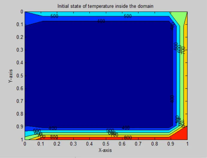
2D Steady State Implicit method analsysis of a square domain (10 grid points) :
By applying laplace equation for 2D steady state heat conduction to the initial temperature domain and solving the governing eqn. PDE by discretising in Implicit method and obtaining solution state by solving for unknowns in linear simulataneous equations form using the Iterative techniques, where guess value are converged itteratively(error) to solution.
1) Selection data :State =1 ,iterative_solver = 1
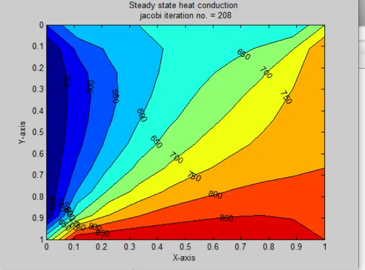
In jacobi as Told values are only used for each convergence loop to obatain T (new) and eventually takes 208 iterations for Told ~ Tnew
2) Selection data :State =1 ,iterative_solver = 2
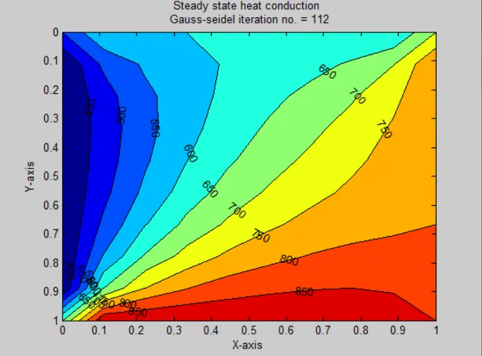
In Gauss-seidel as Told values are updated from prvious calculations for each convergence loop to obatain T (new) and causing it to converge faster than jacobi at only 112 iterations until Told ~ Tnew
3) Selection data :State =1 ,iterative_solver = 3
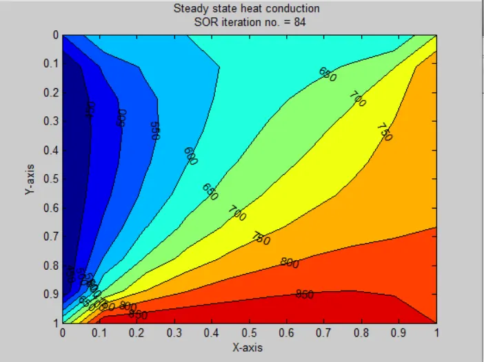
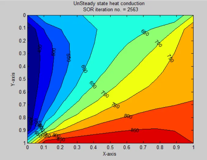
SOR here is applied to Gauss-seidel , Where relaxation factor Omega =1.15 , (>1) reduces the itearations to converge to solution.
2D Unsteady State Explicit method analsysis of a square domain (10 grid points) :
By applying laplace equation for 2D Unsteady state heat conduction to the initial temperature domain and solving the governing eqn. PDE by discretising in Explicit method and obtaining solution state by solving for unknowns using the known values from the neighbouring nodes. Here Time marching rate is restricted or to be within limits to obatain a stable solution.
Selection data :State =2 ,method =1
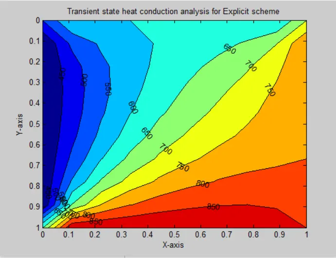
2D Unsteady State Implicit method analsysis of a square domain (10 grid points) :
By applying laplace equation for 2D Unsteady state heat conduction to the initial temperature domain and solving the governing eqn. PDE by discretising in Implicit method and obtaining solution state by solving for unknowns in linear simulataneous equations form using the Iterative techniques, where guess value are converged itteratively(error) to solution.Here as the Time marches in each step T_prev values are updated in the converging equation loop,therefore T_in is converging towards T_final at each & every time steps causing more no. of iteration in total compared to direct steady state iterations.
1) Selection data :State =2 ,method =2,iterative_solver = 1
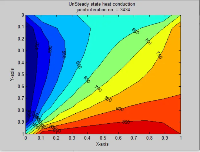
2) Selection data :State =2 ,method =2,iterative_solver = 2
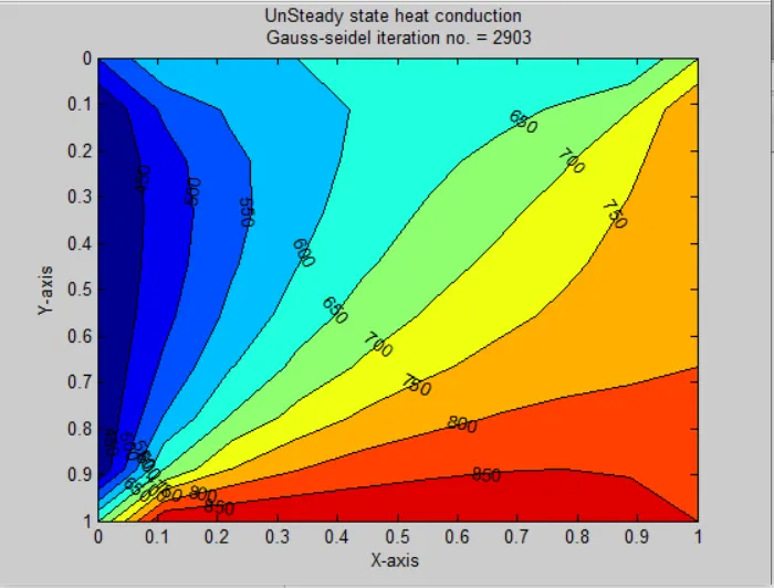
3) Selection data :State =2 ,method =2,iterative_solver = 3