Week 11 - Simulation of Flow through a pipe in OpenFoam
Objective :-
- To simulate an axi-symmetric flow by applying the wedge boundary condition in OpenFoam
- Matlab code to generate blockMeshDict file , which includes input varaints.
- To validate results with the Hagen- Poiseuille's equations for the fully developed flow.
Flow physics given :- The flow is laminar and flows through a constant cross-section pipe at an inlet Reynold's number of 2100.
Solution :-
The fluid motion basically described by two methods based on the fluid properties such as velocity,acceleration, pressure,density,etc. being described & studied.
1) Lagrangian method - a 'single fluid particle' is followed during its motion.
2) Eulerian method - at a 'point' in flow field. (this method is commonly used)
Laminar flow : In laminar flow is defined as that type of in which the fluid particles move along well-definied paths or stream line and all stream line are straight & parallel.Laminar flow is a flow regime characterized by high momentum diffusion and low momentum convection.
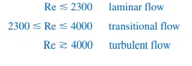
Reynold's no. : The flow regime depends mainly on the ratio of Inertia forces to viscous forces in the fluid.This ratio is called the Reynolds number and is expressed for internal flow in a circular pipe as

Consider a fluid entering a circular pipe at a uniform velocity. Considering no-slip boundary condition at the pipe walls, results of friction a velocity gradient develops along the pipe.The region of the flow in which the effects of the viscous shearing forces caused by fluid viscosity are felt is called the velocity boundary layer and this divides the flow in a pipe into two regions: the boundary layer region, in which the
viscous effects and the velocity changes are significant, and the irrotational (core) flow region, in which the frictional effects are negligible and the velocity remains essentially constant in the radial direction.
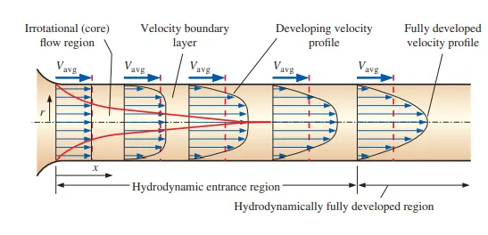
The region from the pipe inlet to the point at which the velocity profile is fully developed is called the hydrodynamic entrance region,
and the length of this region is called the hydrodynamic entry length.Flow in the entrance region is called hydrodynamically developing flow
since this is the region where the velocity profile develops. The region beyond the entrance region in which the velocity profile is fully developed and remains unchanged is called the hydrodynamically fully developed region. The flow is said to be fully developed.
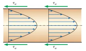
The shear stress at the pipe wall tw is related to the slope of the velocity profile at the surface. Noting that the velocity profile remains unchanged in the hydrodynamically fully developed region, the wall shear stress also remains constant in that region.
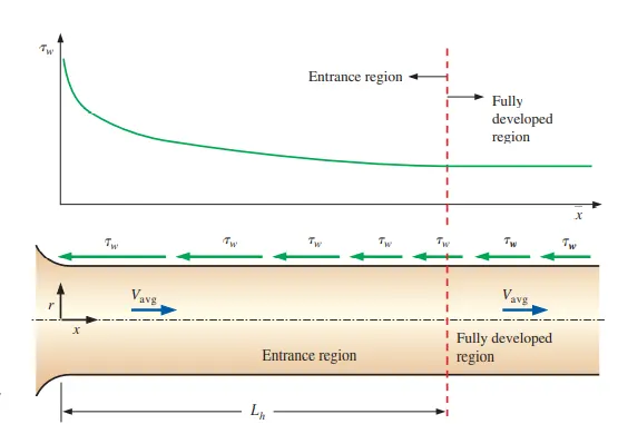
Consider fluid flow in the hydrodynamic entrance region of a pipe. The wall shear stress is the highest at the pipe inlet where the thickness of the boundary layer is smallest, and decreases gradually to the fully developed value.Therefore, the pressure drop is higher in the
entrance regions of a pipe, and the effect of the entrance region is always to increase the average friction factor for the entire pipe. This increase may be significant for short pipes but is negligible for long ones.
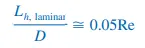
Entry length : In laminar flow, the nondimensional hydrodynamic entry length is given approximately as
Hagen - Poiseuille equation :-
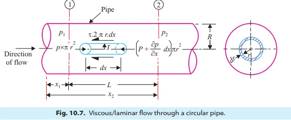
Consider a horizontal pipe of radius 'R',the viscous fluid(water) is flowing through it. consider a small concentric cylinder(fluid element) of radius 'r' and length 'dx'.
shear stress distribution -
While summing the forces(pressure force on left & right face & shear force) acting on the fluid element, we get shear stress
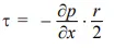 Thus the shear stress across the section varies with 'r' as dp/dx is constant.Hence shear stress distribution across the section is linear.
Velocity distribution -
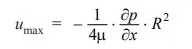
comparing with newton's law of viscosity and integrating velocity gradient , we get 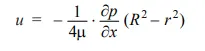
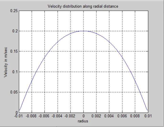
The velocity distribution curve shows parabola, hence the max velocity occurs at the centre.
Ratio of max velocity to average velocity -
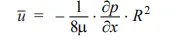
The average velocity is obtained by dividing the discharge of fluid across the section by area of pipe.

above equation shows that average velocity is 1/2 of average velocity. substituting 'Umax'
Drop of pressure for a given length of pipe -
The pressure difference b/w two section 1 & 2 at distance x1 & x2 is given by
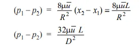 is known as Hagen- Poiseuille's equations.
Input parameter :-
Fluid = Water
density(rho `rho`) = 1000kg/m3
kinematic viscosity(nu `nu`) = 1e-6 m2/sec
dynamic viscosity(mu `mu`) = 1e-3 N-s/m2
Reynold's no. = 2100 (laminar)
Pipe Geometry :-
Length = 2.3m
Diameter = 0.02m ; radius = 0.01m
Hydrodynamic length(Lh) = 0.05 x Reynold's no. x Diameter = 2.1m
Average velocity = (kinematic viscosity x Reynold's no.)/Diameter = 0.105m/sec
Max. velocity = 2 x Average velocity = 0.21 m/sec
OpenFoam Goemetry -
For Axi-symmetric flow by applying the wedge boundary condition,
Wedge angle = 4 degrees.
Matlab code to genrate blockMeshDict file :-
Text File is generated using 'fopen' command & writing done using 'fprintf' command for every line to be printed.
File can be generated in required folder using appropriate navigation & thus can be automated in obtaining CFD results using in Ubuntu software.
clear all
close all
clc

%Inputs of Pipe all are in meters
theta = 4; %degress
Dia = 0.02; % Diameter
r =Dia/2; %Radii
L =2.3; %Length
re =2100; %reynold's no.
Lh =0.05*Dia*re; %Hydrodynamic length
kin_viscosity = 1e-6; %Kineamtic viscosity
velocity_avg = (re*kin_viscosity)/Dia; % Average velocity
CFL = (velocity_avg*0.005)/50; %courant no.

%vertices coordinate points
vz=r*sind(theta/2);
vy=r*cosd(theta/2);

%File writing
f2=fopen('blockmesh.txt','w');
fprintf(f2,'%s\n','/*--------------------------------*- C++ -*----------------------------------*\')
fprintf(f2,'%s\n','  =========                 |')
fprintf(f2,'%s\n','  \\      /  F ield         | OpenFOAM: The Open Source CFD Toolbox')
fprintf(f2,'%s\n','   \\    /   O peration     | Website:  https://openfoam.org')
fprintf(f2,'%s\n','    \\  /    A nd           | Version:  8')
fprintf(f2,'%s\n','     \\/     M anipulation  |')
fprintf(f2,'%s\n','\*---------------------------------------------------------------------------*/')
fprintf(f2,'%s\n','FoamFile')
fprintf(f2,'%s\n','{')
fprintf(f2,'%s\n','   version     2.0;')
fprintf(f2,'%s\n','    format      ascii;')
fprintf(f2,'%s\n','    class       dictionary;')
fprintf(f2,'%s\n','    object      blockMeshDict;')
fprintf(f2,'%s\n','}')
fprintf(f2,'%s\n','// * * * * * * * * * * * * * * * * * * * * * * * * * * * * * * * * * * * * * //')
fprintf(f2,'\n')
fprintf(f2,'%s\n','convertToMeters 0.1;')
fprintf(f2,'%s\n','')
fprintf(f2,'%s\n','vertices')
fprintf(f2,'%s\n','(')
fprintf(f2,'%5s%g %g %g)\n','(',0 ,0 ,0)
fprintf(f2,'%5s%g %g %g) \n','(',0 ,vy ,-vz)
fprintf(f2,'%5s%g %g %g) \n','(',0, vy, vz)
fprintf(f2,'%5s%g %g %g) \n','(',L, 0, 0)
fprintf(f2,'%5s%g %g %g) \n','(',L, vy, -vz)
fprintf(f2,'%5s%g %g %g) \n','(',L, vy, vz)
fprintf(f2,'%s\n',');')
fprintf(f2,'\n')
fprintf(f2,'%s\n','blocks')
fprintf(f2,'%s\n','(')
fprintf(f2,'%7s (%g %g %g %g %g %g %g %g) (%g %g %g) %s (%g %g %g)\n','hex', 0, 1, 2, 0, 3, 4, 5, 3, 50, 1, 100, 'simpleGrading', 1, 1, 1)
fprintf(f2,'%s\n',');')
fprintf(f2,'\n')
fprintf(f2,'%s\n','edges')
fprintf(f2,'%s\n','(')
fprintf(f2,'%7s %g %g (%g %g %g)\n','arc', 1, 2, 0, r, 0)
fprintf(f2,'%7s %g %g (%g %g %g)\n','arc', 4, 5, L, r, 0)
fprintf(f2,'%s\n',');')
fprintf(f2,'\n')
fprintf(f2,'%s\n','boundary')
fprintf(f2,'%s\n','(')
fprintf(f2,'%9s \n','Inlet')
fprintf(f2,'%5s\n','{')
fprintf(f2,'%19s\n','type patch;')
fprintf(f2,'%13s\n','faces')
fprintf(f2,'%9s\n','(')
fprintf(f2,'%13s%g %g %g %g) \n','(', 0, 1, 2, 0)
fprintf(f2,'%10s\n',');')
fprintf(f2,'%5s\n','}')
fprintf(f2,'%10s\n','Outlet')
fprintf(f2,'%5s\n','{')
fprintf(f2,'%19s\n','type patch;')
fprintf(f2,'%13s\n','faces')
fprintf(f2,'%9s\n','(')
fprintf(f2,'%13s%g %g %g %g) \n','(', 3, 5, 4, 3)
fprintf(f2,'%10s\n',');')
fprintf(f2,'%5s\n','}')
fprintf(f2,'%9s\n','front')
fprintf(f2,'%5s\n','{')
fprintf(f2,'%19s\n','type wedge;')
fprintf(f2,'%13s\n','faces')
fprintf(f2,'%9s\n','(')
fprintf(f2,'%13s%g %g %g %g) \n','(', 0, 3, 4, 1)
fprintf(f2,'%10s\n',');')
fprintf(f2,'%5s\n','}')
fprintf(f2,'%8s\n','Back')
fprintf(f2,'%5s\n','{')
fprintf(f2,'%19s\n','type wedge;')
fprintf(f2,'%13s\n','faces')
fprintf(f2,'%9s\n','(')
fprintf(f2,'%13s%g %g %g %g) \n','(', 0, 2, 5, 3)
fprintf(f2,'%10s\n',');')
fprintf(f2,'%5s\n','}')
fprintf(f2,'%16s\n','Topcurvature')
fprintf(f2,'%5s\n','{')
fprintf(f2,'%18s\n','type wall;')
fprintf(f2,'%13s\n','faces')
fprintf(f2,'%9s\n','(')
fprintf(f2,'%13s%g %g %g %g) \n','(', 1, 4, 5, 2)
fprintf(f2,'%10s\n',');')
fprintf(f2,'%5s\n','}')
fprintf(f2,'%12s\n','axisline')
fprintf(f2,'%5s\n','{')
fprintf(f2,'%19s\n','type empty;')
fprintf(f2,'%13s\n','faces')
fprintf(f2,'%9s\n','(')
fprintf(f2,'%13s%g %g %g %g) \n','(', 0, 3, 3, 0)
fprintf(f2,'%10s\n',');')
fprintf(f2,'%5s\n','}')
fprintf(f2,'%s\n',');')
fprintf(f2,'\n')
fprintf(f2,'%s\n','mergePatchPairs')
fprintf(f2,'%s\n','(')
fprintf(f2,'%s\n',');')
fprintf(f2,'\n')
fprintf(f2,'%s\n','// ************************************************************************* //')


fclose(f2);
blockmeshDict file -
- Boundaries at Inlet & outlet are considered as basic patch type, that contains no geometric or topological information about the mesh.
- Boundaries at Back & Front are considered as wedge type, for the given axi-symmetric cases,the geometry is specified as a wedge of small angle (e.g. < 5). and 1 cell thick running along the plane of symmetry, straddling one of the coordinate planes.
- Boundaries at Topcurvature are basic wall function applied (eg. no slip).
- At axis line, as OpenFOAM always generates geometries in 3 dimensions, it can be instruct to solve in 2 (or 1) dimensions by specifying a special empty condition.
- At edges , circular arc is used with two vertices at both sides.
/*--------------------------------*- C++ -*----------------------------------*\
  =========                 |
  \\      /  F ield         | OpenFOAM: The Open Source CFD Toolbox
   \\    /   O peration     | Website:  https://openfoam.org
    \\  /    A nd           | Version:  8
     \\/     M anipulation  |
\*---------------------------------------------------------------------------*/
FoamFile
{
    version     2.0;
    format      ascii;
    class       dictionary;
    object      blockMeshDict;
}
// * * * * * * * * * * * * * * * * * * * * * * * * * * * * * * * * * * * * * //

convertToMeters 1;

vertices
(
    (0 0 0)
    (0 0.00999391 -0.000348995)
    (0 0.00999391 0.000348995)
    (2.3 0 0)
    (2.3 0.00999391 -0.000348995)
    (2.3 0.00999391 0.000348995)
);

blocks
(
    hex (0 1 2 0 3 4 5 3) (50 1 100) simpleGrading (1 1 1)
);

edges
(
    arc 1 2 (0 0.01 0)
    arc 4 5 (2.3 0.01 0)
);

boundary
(
    Inlet
    {
        type patch;
        faces
        (
            (0 1 2 0)
        );
    }
    Outlet
    {
        type patch;
        faces
        (
            (3 5 4 3)
        );
    }
    front
    {
        type wedge;
        faces
        (
            (0 3 4 1)
        );
    }
    Back
    {
        type wedge;
        faces
        (
            (0 2 5 3)
        );
    }
    Topcurvature
    {
        type wall;
        faces
        (
            (1 4 5 2)
        );
    }
    axisline
    {
        type empty;
        faces
        (
            (0 3 3 0)
        );
    }
);

mergePatchPairs
(
);

// ************************************************************************* //
Initial conditions :
Pressure - At Inlet face & Topcurvature Normal gradient of preesure is zero (constant pressure). At outlet face the gradient is specified,Drichlet BC(specific value set to zero).
Note : Here in icoFoam pressure is normalized by density called Kinematic pressure.
/*--------------------------------*- C++ -*----------------------------------*\
  =========                 |
  \\      /  F ield         | OpenFOAM: The Open Source CFD Toolbox
   \\    /   O peration     | Website:  https://openfoam.org
    \\  /    A nd           | Version:  8
     \\/     M anipulation  |
\*---------------------------------------------------------------------------*/
FoamFile
{
    version     2.0;
    format      ascii;
    class       volScalarField;
    object      p;
}
// * * * * * * * * * * * * * * * * * * * * * * * * * * * * * * * * * * * * * //

dimensions      [0 2 -2 0 0 0 0];

internalField   uniform 0;

boundaryField
{
    Inlet
    {
        type            zeroGradient;
    }

    Outlet
    {
        type           fixedValue;
        value	        uniform 0;
    }

    front
    {
        type            wedge;
    }
    Back
    {
        type            wedge;
    }
    Topcurvature
    {
        type            zeroGradient;
    }
    axisline
    {
        type            empty;
    }
}

// ************************************************************************* //
Velocity- velocity is expressed by 3 vector components. The internal field is initialised as uniform zero.
When the flow is inwards it is 'fixedValue',i.e Normal gradient is specified (at x-component of U).
When the flow is inwards it is 'fixedValue',i.e Normal gradient is zero (constant). where the values are calculated as time marches to end grids from where it is extrapolated. At top curvature no-slip condition is applied(viscous flow).
/*--------------------------------*- C++ -*----------------------------------*\
  =========                 |
  \\      /  F ield         | OpenFOAM: The Open Source CFD Toolbox
   \\    /   O peration     | Website:  https://openfoam.org
    \\  /    A nd           | Version:  8
     \\/     M anipulation  |
\*---------------------------------------------------------------------------*/
FoamFile
{
    version     2.0;
    format      ascii;
    class       volVectorField;
    object      U;
}
// * * * * * * * * * * * * * * * * * * * * * * * * * * * * * * * * * * * * * //

dimensions      [0 1 -1 0 0 0 0];

internalField   uniform (0 0 0);

boundaryField
{
    Inlet
    {
        type            fixedValue;
        value           uniform (0.105 0 0);
    }

    Outlet
    {
        type            zeroGradient;
    }

    front
    {
        type            wedge;
    }
    Back
    {
        type            wedge;
    }
    Topcurvature
    {
        type            noSlip;
    }
    axisline
    {
        type            empty;
    }
}

// ************************************************************************* //
controlDict file -
Input data relating to the control of time and reading and writing of the solution data are read in from the controlDict dictionary
The total simulation time = time step x end time = 0.001x10=0.01seconds. At which the flow attains the steady state.
To achieve accuracy and numerical stability when running icoFoam, a Courant number of less than 1 is required. The Courant number is defined for one cell as: Co =dt|U|/dx. The flow velocity varies across the domain and we must ensure Co < 1 everywhere.
/*--------------------------------*- C++ -*----------------------------------*\
  =========                 |
  \\      /  F ield         | OpenFOAM: The Open Source CFD Toolbox
   \\    /   O peration     | Website:  https://openfoam.org
    \\  /    A nd           | Version:  8
     \\/     M anipulation  |
\*---------------------------------------------------------------------------*/
FoamFile
{
    version     2.0;
    format      ascii;
    class       dictionary;
    location    "system";
    object      controlDict;
}
// * * * * * * * * * * * * * * * * * * * * * * * * * * * * * * * * * * * * * //

application     icoFoam;

startFrom       startTime;

startTime       0;

stopAt          endTime;

endTime         10;

deltaT          0.001;

writeControl    timeStep;

writeInterval   20;

purgeWrite      0;

writeFormat     ascii;

writePrecision  6;

writeCompression off;

timeFormat      general;

timePrecision   6;

runTimeModifiable true;


// ************************************************************************* //
transportProperties -
For an icoFoam case, the only property that must be specified is the kinematic viscosity(`nu`) in transportProperties dictionary.
/*--------------------------------*- C++ -*----------------------------------*\
  =========                 |
  \\      /  F ield         | OpenFOAM: The Open Source CFD Toolbox
   \\    /   O peration     | Website:  https://openfoam.org
    \\  /    A nd           | Version:  8
     \\/     M anipulation  |
\*---------------------------------------------------------------------------*/
FoamFile
{
    version     2.0;
    format      ascii;
    class       dictionary;
    location    "constant";
    object      transportProperties;
}
// * * * * * * * * * * * * * * * * * * * * * * * * * * * * * * * * * * * * * //

nu              [0 2 -1 0 0 0 0] 0.000001;


// ************************************************************************* //
Praview Mesh view -
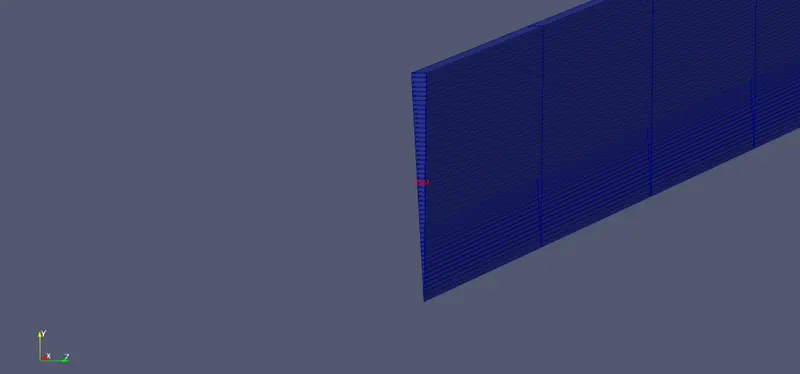
Now to verify the blockmeshDict file , we need to run in terminal using ''blockMeshDict' command & after succesful execution should 'checkMesh' command, which will confim the mesh geometry details.
The mesh is then viewed in paraFoam, the post-processing tool supplied with OpenFOAM.The paraFoam post-processing is started by typing in the terminal from within the case directory.
Along Y-axis there is only unit element considered for 2D analysis.
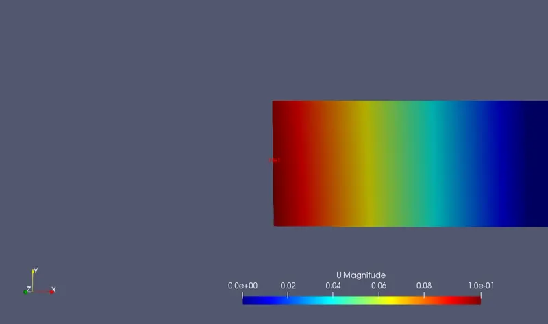
Initial Velocity distribution -
The Intial velocity condition at time,t=0
Final Velocity distribution at the Inlet of pipe -
At time = final or steady state , below is the velocity contour view at Inlet of pipe flow.
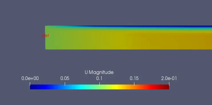
Using plot over line option we can get below results -
Apply PlotOverLine, in which the user can specify the end points of the line in the Properties panel.
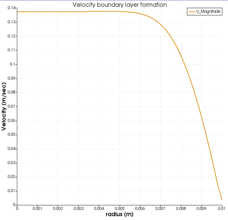
From above plot at length=0.01m we can observe that boundary layer formation within hydrodynamic entrance region , in which the viscous effects and the velocity changes are significant at the wall.
Final Velocity distribution at the Outlet of pipe -
At time = final or steady state , below is the Uvelocity contour view at Outlet of pipe flow.
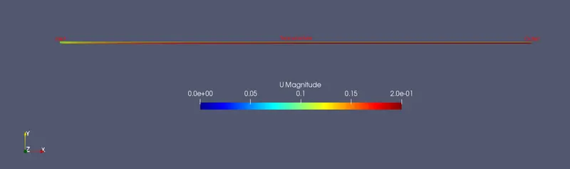
It is clear from the simulation that the max velocity attained at axis of pipe in fully developed flow region.
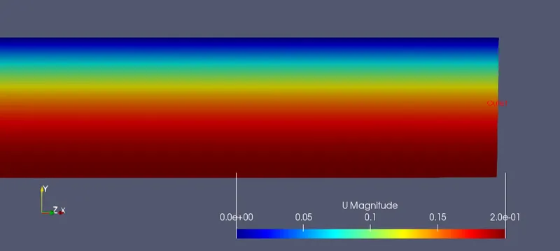
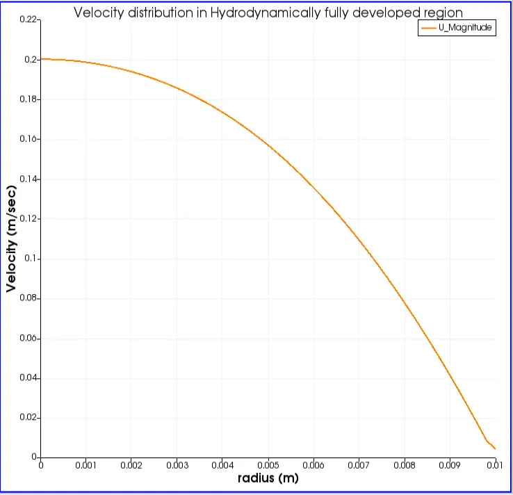
At length =2.08m At length =2.3m
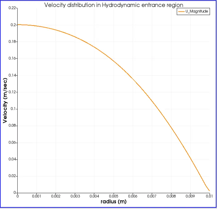
From above plot at length=2.08m is the developing flow region , where it is almost approached full velocity prabolic profile. The thickness of boundary layer increases in the flow direction until the laminar boundary layer reaches the pipe center and thus fills the entire pipe.
From above plot at length=2.3m at end of pipe , where flow is fully developed. At length 2.1m velocity becomes fully developed and gradient of velocity remains constant radially.
Velocity distribution throughout the pipe -
Pressure distribution throughout the pipe -
Pressure drop is clearly visible in this final steady state pressure contour throughout the lenght of pipe.
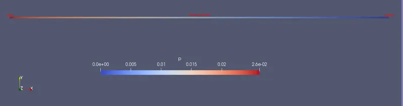
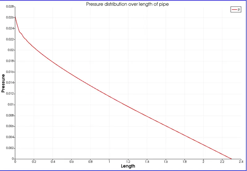
The pressure drop is higher in the entrance regions of a pipe, and the effect of the entrance region is always to increase the average friction factor for the entire pipe.
Matlab code to evalute shear stress analytically
In the fully developed flow region of a pipe, the velocity profile does not change downstream, and thus the wall shear stress remains constant as well. At Fully developed region (L=2.3m) will extract the plot data from export Spread sheet view option to a text file, this data consists of U components,points & arc length etc.
Below program evaluates the shear stress using Newtons Law viscosity & values extracted from U-plot.
clear all
close all
clc

%File reading

f4=fopen('points_Y.txt','r')

%File extracting
a=fgetl(f4);

%Using Delimiter to access integer divided by comma
c=textscan(f4,'%f %f %f %f %f %f %f %f %f %f', 'Delimiter',',');

u=c{1}; %Velocity X component(magnitude)
arc=c{6}; % Arc length
tou=zeros(1,1001); %  Intialize array - shear stress

%Dynamic viscosity
mu = 1e-6;


for i=2:1001
    %Newtons viscocity formulae for fing viscous shear sress
    tou(i)= ((u(i-1)-u(i))/(arc(i)-arc(i-1)))*mu;

end


figure(1)  %shear stress plot over the dia
plot(arc,tou)
hold on
plot(-arc,tou)
grid on
xlabel('radius')
ylabel('Shear stress in N/m2')
title('Shear stress distribution along radial distance')

figure(2) %Velocity distribution plot
plot(arc,u)
hold on
plot(-arc,u)
grid on
xlabel('radius')
ylabel('Velocity in m/sec')
title('Velocity distribution along radial distance')
Shear stress distribution along the Pipe Diameter -Analytical result
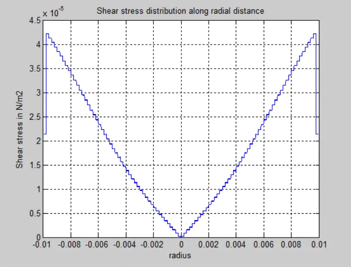
From above plot it is evaluated that shear stree varies linearly accross the section/diameter.
Velocity distribution along the Pipe Diameter - Analytical results
Full section profile view of velocity in below plot
Matlab code to evalute kinematic pressure :-
In OpenFoam dimension specified for pressure is kinematic pressure.
Kinematic pressure = 
The SI unit of P is m2/s2Kinematic pressure is used in the same manner as kinematic viscosity in order to compute the Navier–Stokes equation without explicitly showing the density.
Below code results shows evaluation or comaparision of Numerical & calculated/analytical kinematic pressure. Using the data (.txt format) extracted from post-processor. (pressure,arc length)
Here, fully developed region(L= 2.2m to 2.25m) is considered for analysis ,as in this region pressure drop remains constant.
clear all
close all
clc

%File reading
fpp=fopen('Pressure22to225.txt','r')

%File extracting
a=fgetl(fpp);

%Input constants
nu= 1e-3; %Kinematic viscosity
v_avg=0.1050; % Average velocity
r=0.01; %Radius

%Using Delimiter to access index by eleminating comma
c=textscan(fpp,'%f %f %f %f64 %f %f %f %f %f %f', 'Delimiter',',');

p=c{4};% kinematic Pressure from OpenFoam results
arc=c{6}; %arc length or lenght of pipe from 2.2m to 2.25m

%  Intialize array
Kin_pr_numerical=zeros(1,1001);
Kin_pr_analytical=zeros(1,1001);

for i=2:1001
    %Numerical Kinematic pressure difference/drop
    Kin_pr_numerical(i)= (p(i-1)-p(i));
    %Analytical pressure difference/drop
    pr_gradient(i) = ((8*nu*v_avg)/(r^2))*(arc(i-1)-arc(i));
    Kin_pr_analytical(i)=-pr_gradient(i)/1000;  %Analytical Kinematic pressure
    %Error
    error(i) = Kin_pr_numerical(i)-Kin_pr_analytical(i);
end


%Pressure drop plot both methods
figure(1)
plot(arc,Kin_pr_numerical)
hold on
plot(arc,Kin_pr_analytical,'r')
xlabel('Fully developed region Length(2.2m to 2.25m)')
ylabel('Kinematic pressure gradient')
title('Kinematic pressure gradient variation along length')
legend('Numerical Kinematic pressure','Analytical Kinemati pressure')

%Evaluating the pressure drop
figure(2)
plot(arc,error)
xlabel('Fully developed region Length')
ylabel('Error')
title('Error Numerical results vs Analytical results')
Pressure gradient is calculated using Hagen- Poiseuille's equations for the fully developed flow and then divided by density to get the kinematic pressure analytical.
Comparision of kinematic pressure analytically vs numerical
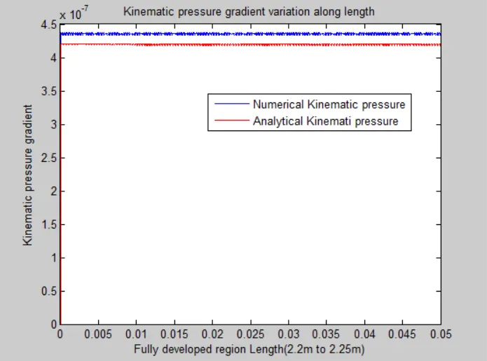
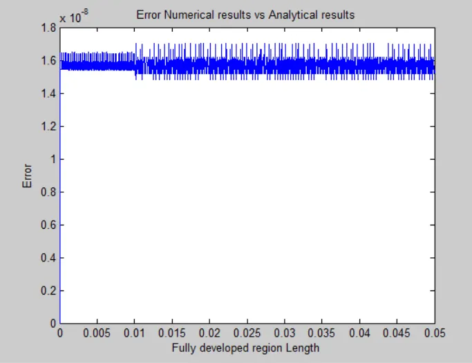
We can can observe that there is a minimal variation/difference b/w the results of analytical & Numerical CFD values.
References :-
- standard boundary condition reference - https://www.openfoam.com/documentation/user-guide/standard-boundaryconditions.php#x35-138000A.4
- Fluid mechanics by Cengel Yunus A.