Week 3.5 - Deriving 4th order approximation of a 2nd order derivative using Taylor Table method

function [Central_difference_error, right_sided_difference_error, left_sided_difference_error] = second_order_fourth_approximation(x,dx)

%Evaluation of the second-order derivative of the analytical function
%vs 4th order approximations 

% Co-efficents obtained from Taylor's table method for different scheme 
%4th order accuracy/approximation

%Skewed left-sided difference 
L=[1 1 1 1 1 1;-5 -4 -3 -2 -1 0;25/2 8 9/2 2 1/2 0;-125/6 -64/6 -27/6 -4/3 -1/6 0;125*5/24 64/6 27/8 2/3 1/24 0;-125*25/120 -64*16/120 -27*9/120 -32/120 -1/120 0];
%Skewed right-sided difference
R=[1 1 1 1 1 1;5 4 3 2 1 0;25/2 8 9/2 2 1/2 0;125/6 64/6 27/6 4/3 1/6 0;125*5/24 64/6 27/8 2/3 1/24 0;125*25/120 64*16/120 27*9/120 32/120 1/120 0];
%Central difference 
C=[1 1 1 1 1;-2 -1 0 1 2;2 1/2 0 1/2 2;-8/6 -1/6 0 1/6 8/6;16/24 1/24 0 1/24 16/24];
%Solving for system of equation of unknown co-efficients % Let
BLR =[0;0;1;0;0;0]; % 6 Nodes in stencil for one sided 
BC = [0;0;1;0;0];  % 5 Nodes in stencil for central 
% using the matrix inversion method to solve equations directly
cd_coefficients = C\BC; % Central difference co-efficients [d;e;g;h;k] 
skewed_coefficients = R\BLR; %Skewed right[o;n;m;k;h;g] & left[a;b;c;d;e;g] sided co-efficients are same



%analytical_derivative is f''(x)= -2*exp(x)*sin(x)
analytical_derivative =  -2*exp(x)*sin(x);

% Finite difference equation for 4th order approximations of the second-order derivative

%Central_difference=(d*f(x-2*dx)+e*f(x-dx)+g*f(x)+h*f(x+dx)+k*f(x+2*dx))/dx^2
% As co-efficients are in array,Let ([f(x-2*dx) f(x-dx) f(x) f(x+dx) f(x+2*dx)]*cd_coefficients)/dx^2
Central_difference = ([exp(x-2*dx)*cos(x-2*dx) exp(x-dx)*cos(x-dx) exp(x)*cos(x) exp(x+dx)*cos(x+dx) exp(x+2*dx)*cos(x+2*dx)]*cd_coefficients)/dx^2;

%Skewed right-sided difference=(g*f(x)+h*f(x+dx)+k*f(x+2*dx)+m*f(x+3*dx)+n*f(x+4*dx)+o*f(x+5*dx))/dx^2
% As co-efficients are in array,Let ([f(x+5*dx) f(x+4*dx) f(x+3*dx) f(x+2*dx) f(x+dx) f(x)]*skewed_coefficients)/dx^2
right_sided_difference = ([exp(x+5*dx)*cos(x+5*dx) exp(x+4*dx)*cos(x+4*dx) exp(x+3*dx)*cos(x+3*dx) exp(x+2*dx)*cos(x+2*dx) exp(x+dx)*cos(x+dx) exp(x)*cos(x)]*skewed_coefficients)/dx^2;

%Skewed left-sided difference=(g*f(x)+e*f(x-dx)+d*f(x-2*dx)+c*f(x-3*dx)+b*f(x-4*dx)+a*f(x-5*dx))/dx^2
% As co-efficients are in array,Let ([f(x-5*dx) f(x-4*dx) f(x-3*dx) f(x-2*dx) f(x-dx) f(x)]*skewed_coefficients)/dx^2
left_sided_difference = ([exp(x-5*dx)*cos(x-5*dx) exp(x-4*dx)*cos(x-4*dx) exp(x-3*dx)*cos(x-3*dx) exp(x-2*dx)*cos(x-2*dx) exp(x-dx)*cos(x-dx) exp(x)*cos(x)]*skewed_coefficients)/dx^2;

%Error in each scheme
Central_difference_error = abs(Central_difference-analytical_derivative)
right_sided_difference_error = abs(right_sided_difference-analytical_derivative)
left_sided_difference_error = abs(left_sided_difference-analytical_derivative)

end

Above program creates a function with 3 outputs [Central_difference_error, right_sided_difference_error, left_sided_difference_error] and inputs (x,dx). Here co-efficients answers are directlty in-corporated into solution equation in an array and values are in decimals.

Now this function is called in below program over the range of dx(discrete points)

clear all
close all
clc
x=pi/3;
dx = linspace(pi/300,pi/50,20);
for i = 1:length(dx)
   dx(i)
    [Central_difference_error(i),right_sided_difference_error(i),left_sided_difference_error(i)]=second_order_fourth_approximation(x,dx(i));
    
end

figure(1)
loglog(dx,Central_difference_error,'g*-')
hold on
loglog(dx,right_sided_difference_error,'b-o')
hold on
loglog(dx,left_sided_difference_error,'+-r')
legend('Central difference of 4th order','right sided difference of 4th order','left sided difference of 4th order')
xlabel('dx/discrete points/mesh size');
ylabel('Abs Error value');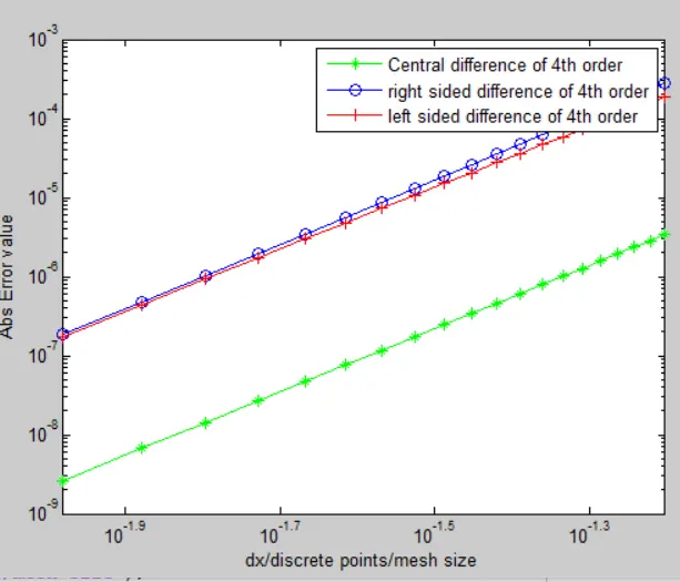

above plot clearly shows that with same 4th order accuracy of the derived second order derivative the abs.error of

central difference <right-sided difference<left sided difference.

Question - In your own words, describe why a skewed scheme is useful? What can a skewed scheme do that a CD scheme cannot?

Answer : Skewed scheme useful particularly in boundary region, where differencing is possible only in one direction, i.e away from boundary. Here central difference fails because another point beneath the boundary & it is outside the domain of computation & we have no info.