Week 7 - Simulation of a 1D Super-sonic nozzle flow simulation using Macormack Method
Objective :- Simulation of a 1D Super-sonic nozzle flow simulation using Macormack Method.
Solution :-
We consider the steady,isentropic flow through a convergent-divergent nozzle as sketched below. The at Inlet comes from a large reservoir where pressure p0 & temperature T0 respectively. The cross-sectional area is very large , hence velocity V0 is very small. The flow expands isentropically to supersonic speed at the nozzle exit and it is locally subsonic in the convergent section & sonic at throat.
In reality the flow field is 2 dimensional but we make assumptions that the flow properties vary only in x direction, such a flow is termed as quasi-one-dimensional flow.
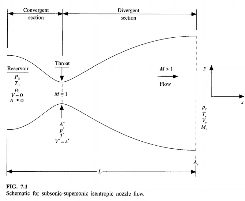
The governing continuity, momentum and energy equations for this quasi-one-dimensional steady isentropic flow can be expressed as below
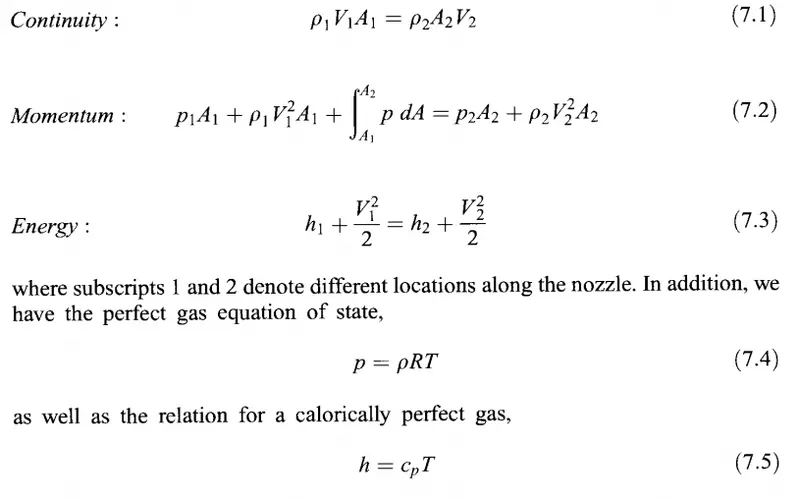
These equations can be solved to get the exact analytical solution.
Governing Flow equations :
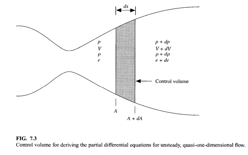
When we apply the integral form of x-component of the governing equations of inviscid flow to the above shaded control volume (with infinitesimal thickness dx) we end up with PDE's and when it is represented in non-dimensional variables
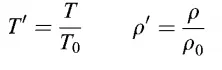


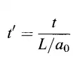

Conservation form -
1) Continuity equation : 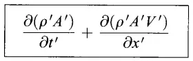
2) Momentum equation :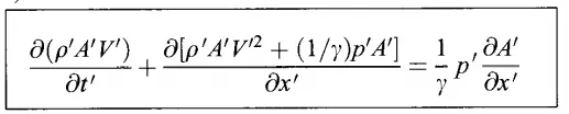
3)Energy equation : 
Non -Conservation form -
1) Continuity equation : 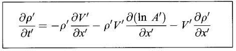
2) Momentum equation : 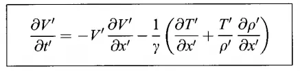
3)Energy equation : 
In conservation form we can solve by expressing in solution vector 'U' and flux vector 'F' and source term as 'J'
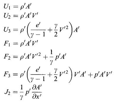
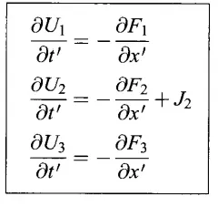
With this elements , we can represent our conservation form governing equations as
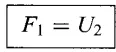
For solving the setup is done in such a way that to get accurate pure form of result we express U in terms F,we get
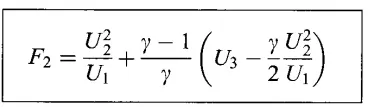
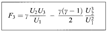
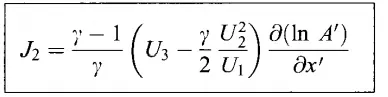
Boundary condition - assuming as 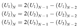
Intial conditions - in relation to length of nozzle 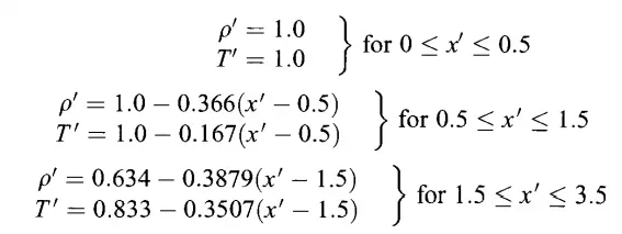
Non-conservative solver code :
 function [rho,v,T,p,M,m,rho_t,T_t,p_t,M_t]=non_conservative(x,a,nt,gama,n,CFL)


%grid spacing
dx =x(2)-x(1);

%Non-dimensional primitive varaibles
%At t=0 , Assuming linear varaition of varaibles as f(x)
rho =1-0.3146*x; %rho=density
T =1-0.2314*x; %T=temperature
v=(0.1+1.09*x).*T.^0.5; %v=velocity

p=rho.*T; %Pressure
M = v./(T.^0.5); %Mach No.

% %Intial variation plot,at t=0
% figure(1)
% subplot(4,1,1)
% plot(x,rho)
% ylabel('rho')
% title('Intial variation of flow variables Non-Conservative, At t=0')
% subplot(4,1,2)
% plot(x,T)
% ylabel('T')
% subplot(4,1,3)
% plot(x,v)
% ylabel('v')
% subplot(4,1,4)
% plot(x,M)
% ylabel('Mach no.(M)')
% xlabel('Nondimensional distance through nozzle(x)')


%Stability contraint time step value
dt=min(CFL*dx./((T.^0.5)+v));


 %Normalized mass flow rate
m=rho.*v.*a;

figure(2)%Mass flow distribution plot
plot(x,m,'r')
xlabel('X-axis grid space over length of nozzle, x/L ')
ylabel('Mass flow rate, m')
title ({'Variation of mass flow distribution throught the'; 'Nozzle at different time steps- Non Conservative form'})
hold on


%Outer time loop
for k=1:nt
    %Store previous time step values
     rho_old=rho;
     v_old=v;
     T_old=T;


    %predictive method

    for j=2:n-1
        %drho_dt_p = -rho(j)*((v(j+1)+v(j))/dx)-rho(j)*v(j)*log(a(j+1)-a(j))/dx-v(j)*(rho(j+1)-rho(j))/dx
    dvdx=(v(j+1)-v(j))/dx;
    drhodx=(rho(j+1)-rho(j))/dx;
    dTdx=(T(j+1)-T(j))/dx;
    dlog_adx = (log(a(j+1))-log(a(j)))/dx;
      %continuity equation
    drhodt_p(j) = -rho(j)*dvdx-(rho(j)*v(j)*dlog_adx)-(v(j)*drhodx);

    %Momentum equation
    dvdt_p(j) = -v(j)*dvdx - (1/gama)*(dTdx+(T(j)/rho(j))*drhodx);

    %Energy equation
    dTdt_p(j) = -v(j)*dTdx -((gama-1)*T(j)*(dvdx+v(j)*dlog_adx));


     %solution update
     v(j) =v(j)+dvdt_p(j)*dt;
     T(j)=T(j)+dTdt_p(j)*dt;
     rho(j)=rho(j)+drhodt_p(j)*dt;
    end

     %corrector method

    for j=2:n-1
        %drho_dt_p = -rho(j)*((v(j+1)+v(j))/dx)-rho(j)*v(j)*log(a(j+1)-a(j))/dx-v(j)*(rho(j+1)-rho(j))/dx
    dvdx=(v(j)-v(j-1))/dx;
    drhodx=(rho(j)-rho(j-1))/dx;
    dTdx=(T(j)-T(j-1))/dx;
    dlog_adx = (log(a(j))-log(a(j-1)))/dx;
      %continuity equation
    drhodt_c(j) = -(rho(j)*dvdx)-(rho(j)*v(j)*dlog_adx)-(v(j)*drhodx);

    %Momentum equation
    dvdt_c(j) = -(v(j)*dvdx)- (1/gama)*(dTdx+(T(j)/rho(j))*drhodx);

    %Energy equation
    dTdt_c(j) = -v(j)*dTdx -((gama-1)*T(j)*(dvdx+v(j)*dlog_adx));

    end
   %compute the avg time derivative
   dvdt = 0.5*(dvdt_c+dvdt_p);
   drhodt=0.5*( drhodt_c+ drhodt_p);
   dTdt=0.5*( dTdt_c+ dTdt_p);

    %Final solution update

    for i=2:n-1
    v(i) =v_old(i)+dvdt(i)*dt;
     T(i)=T_old(i)+dTdt(i)*dt;
     rho(i)=rho_old(i)+drhodt(i)*dt;
    end

    %Apply boundary condition
    %Inlet BC %subsonic
     v(1) = 2*v(2)-v(3);


     %Outlet %supersonic
     v(n) =(2*v(n-1))-v(n-2);
       rho(n) =(2*rho(n-1))-rho(n-2);
         T(n) =(2*T(n-1))-T(n-2);


  %Other updated flow variables
 p=rho.*T;
 M = v./(T.^0.5);
 m=rho.*v.*a;

   %At n=16, is throat centre variables
   rho_t(k)=rho(16);
   T_t(k)=T(16);
   p_t(k)=p(16);
   M_t(k)=M(16);


figure(2) %mass flow plot
if k==50
    plot(x,m,'--')
    pause(0.03)
    hold on
end
if k==100
    plot(x,m,'k')
    pause(0.03)
    hold on
end
if k==200
    plot(x,m,'g')
    pause(0.03)
    hold on
end
if k==700
   plot(x,m,'+')
   pause(0.03)
   legend('0','50','100','200','700')
end

end


end
Conservative solver code :-
 function [rho,v,T,p,M,u2,rho_t,T_t,p_t,M_t]=conservative(x,a,nt,gama,n,CFL)


 %grid spacing
dx =x(2)-x(1);


%Initial conditions
%Non-dimensional variables
rho =zeros(1,n);%Dummy array
T =zeros(1,n);%Dummy array

%Non-dimensional primitive varaibles
%At t=0 , Assuming linear varaition of varaibles as f(x)
%Convergent subsonic portion
 rho(logical(0<=x & x<=0.5)) =1.0;%Density
 T(logical(0<=x & x<=0.5)) =1.0;%temperature
 %Throat sonic portion
 xi=(logical(0.5<=x & x<=1.5));
rho(xi) =1.0-0.366*(x(xi)-0.5);
T(logical(xi)) =1.0-0.167*(x(xi)-0.5);
%Divergent supersonic portion
 xii=(logical(1.5<=x & x<=3.5));
rho(xii) =0.634-0.3879*(x(xii)-1.5);
T(logical(xii)) =0.833-0.3507*(x(xii)-1.5);

%velocity throughout nozzle assuming constant u2
v=0.59./(rho.*a);

p=rho.*T; %Pressure
M = v./(T.^0.5); %Mach No.

dt=min(CFL*dx./((T.^0.5)+v));

% %Intial variation plot,at t=0
% figure(10)
% subplot(4,1,1)
% plot(x,rho)
% ylabel('rho')
% title('Intial variation of flow variables conservative form, At t=0')
% subplot(4,1,2)
% plot(x,T)
% ylabel('T')
% subplot(4,1,3)
% plot(x,v)
% ylabel('v')
% subplot(4,1,4)
% plot(x,M)
% ylabel('Mach no.(M)')
% xlabel('Nondimensional distance through nozzle(x)')


 %Initial conditions for solution vectors
 u1=rho.*a;
 u2=rho.*a.*v; %Normalized mass flow rate
 u3=rho.*((T./(gama-1))+(gama/2.*v.^2)).*a;

figure(21)
plot(x,u2,'r')
xlabel('X-axis grid space over length of nozzle, x/L ')
ylabel('Mass flow rate, u2=rho*v*a')
title ({'Variation of mass flow distribution throught the';'Nozzle at different time steps - Conservative form'})
hold on


%Outer time loop
for k=1:nt;

% storing old values
u1_old =u1;
u2_old= u2;
u3_old= u3;

   for j=1:n
       %Calculating Intial Flux vectors
       f1(j)=u2(j);
       f2(j)=(u2(j)^2/u1(j))+((gama-1)/gama)*(u3(j)-((gama/2)*(u2(j)^2/u1(j))));
       term2=gama*((gama-1)/2)*(u2(j)^3/u1(j)^2);
       f3(j)= (gama*u2(j)*u3(j))/u1(j)-term2;
       %j22(j)=((gama-1)/gama)*(u3(j)-((gama/2)*(u2(j)^2/u1(j))))*((log(a(j+1))-log(a(j)))/dx);

   end
         %Predictor derivatives - forward differencing
    for j=2:n-1 %Inner nodes
        j2(j) = (1/gama)*rho(j)*T(j)*((a(j+1)-a(j))/dx);

             %continuity equation
       du1dt_p(j)= -(f1(j+1)-f1(j))/dx;
           %Momentum equation
       du2dt_p(j)= j2(j)-((f2(j+1)-f2(j))/dx) ;
          %Energy equation
        du3dt_p(j)= -(f3(j+1)-f3(j))/dx;

         %Predicted solution vector update
         u1(j)= u1(j)+du1dt_p(j)*dt;
         u2(j)=u2(j)+du2dt_p(j)*dt;
         u3(j)=u3(j)+du3dt_p(j)*dt;

         %primitive variables update
         rho_p(j)=u1(j)/a(j);
         term1=(u3(j)/u1(j))-((gama/2)*((u2(j)/u1(j))^2));
         T_p(j)=(gama-1)*term1;
    end
    for j=1:n
         %Predicted flux vector update
       f1(j)=u2(j);
       f2(j)=(u2(j)^2/u1(j))+((gama-1)/gama)*(u3(j)-((gama/2)*(u2(j)^2/u1(j))));
       term2=gama*((gama-1)/2)*(u2(j)^3/u1(j)^2);
       f3(j)= (gama*u2(j)*u3(j))/u1(j)-term2;
     % j2(j) = (1/gama)*rho_p(j)*T_p(j)*((a(j)-a(j-1))/dx);
   end

   %corrector derivatives - backward differencing
     for i=2:n-1
            j2(i) = (1/gama)*rho_p(i)*T_p(i)*((a(i)-a(i-1))/dx);
            %continuity equation
       du1dt_c(i)= -(f1(i)-f1(i-1))/dx;
           %Momentum equation
       du2dt_c(i)= j2(i)-((f2(i)-f2(i-1))/dx);
          %Energy equation
        du3dt_c(i)= -(f3(i)-f3(i-1))/dx;

     end

   %Average time derivative
   du1dt =0.5*(du1dt_c+du1dt_p);
    du2dt =0.5*(du2dt_c+du2dt_p);
    du3dt =0.5*(du3dt_c+du3dt_p);

    %corrected final values

    for i =2:n-1

        u1(i)=u1_old(i)+du1dt(i)*dt;
        u2(i)=u2_old(i)+du2dt(i)*dt;
        u3(i)=u3_old(i)+du3dt(i)*dt;


    end

    %Apply boundary condition (float varaibles)
    %Inlet BC - subsonic
    %By Linear extrapolation
    u2(1)=2*u2(2)-u2(3);
    v(1)=u2(1)/u1(1);
     u3(1)=u1(1)*((T(1)/(gama-1))+(gama/2*v(1)^2));


      %Outlet BC - supersonic
    %By Linear extrapolation
         u1(n) =2*u1(n-1)-u1(n-2);
         u2(n) =2*u2(n-1)-u2(n-2);
         u3(n) =2*u3(n-1)-u3(n-2);

 %final prmitive variables
          rho=u1./a;
         term1= (u3./u1)-((gama/2)*((u2./u1).^2));
         T=(gama-1)*term1;
         v=u2./u1;

 %Other updated flow variables
 p=rho.*T;
 M = v./(T.^0.5);
 u2=rho.*a.*v;

   %At n=16, is throat centre variables
   rho_t(k) =rho(16);
   T_t(k)=T(16);
   p_t(k)=p(16);
   M_t(k)=M(16);


figure(21) %mass flow plot
if k==50
    plot(x,u2,'--')
    pause(0.03)
    hold on
end
if k==100
    plot(x,u2,'k')
    pause(0.03)
    hold on
end
if k==200
    plot(x,u2,'g')
    pause(0.03)
    hold on
end
if k==700
   plot(x,u2,'+')
   pause(0.03)
  legend('0','50','100','200','700')
end

end

 end
Exact analytical solver code using Mach no. relation
function [p,rho,T,M] = analystical_form_solution(x,a)

%% INPUTS

g   = 1.4;
gm1 = g-1;
gp1 = g+1;

th = find(a==1);


% Error tolerance
errTol = 1e-6;

for i = 1:length(a)
%% MATLAB SOLVER

% FZero solver structure
problem.objective = @(M) (1/M^2)*(((2+gm1*M^2)/gp1).^(gp1/gm1))-a(i)^2;     % Objective function
problem.solver    = 'fzero';                                                % Solver Name
problem.options   = optimset(@fzero);                                       % Default options


%Solve subsonic root
if ith
problem.x0 = [1+1e-4 5];
M(i)       = fzero(problem);


end
end
end


%% Primitive variables

p = (1 + (gm1/2).*M.^2).^(-g/gm1);
rho = (1 + (gm1/2).*M.^2).^(-1/gm1);
T =  (1 + (gm1/2).*M.^2).^-1;


end
end
Main functional comparision code :-
close all
clear all
clc

%Non dimensional Inputs
n=31; %no. of grid points
x=linspace(0,3,n);  %1D array space

%Claculate initial profiles of convergent-divergent nozzle
%At x=1.5 is throat centre
a = 1+2.2*(x-1.5).^2; %area


%time steps
nt =1400;


%stability consideration
CFL=0.5; %courant no.
gama =1.4; %specific heat ratio

%Non conservation form solution function
[rho_nc,v_nc,T_nc,p_nc,M_nc,m_nc,rho_tnc,T_tnc,p_tnc,M_tnc]=non_conservative(x,a,nt,gama,n,CFL);

%conservation form solution function
[rho_c,v_c,T_c,p_c,M_c,u2,rho_tc,T_tc,p_tc,M_tc]=conservative(x,a,nt,gama,n,CFL);

%Exact analystical form solution function
[p,rho,T,M] =analystical_form_solution(x,a);


%Steady-state distribution of primitive variables inside the nozzle
figure(11)
subplot(5,1,1)
plot(x,rho_nc,'g')
hold on
plot(x,rho_c,'*')
title('Steady-state distribution of primitive variables inside the nozzle')
ylabel('Density')
subplot(5,1,2)
plot(x,T_nc)
hold on
plot(x,T_c,'*')
ylabel('Temperature')
subplot(5,1,3)
plot(x,v_nc,'g')
hold on
plot(x,v_c,'*')
ylabel('velocity')
subplot(5,1,4)
plot(x,p_nc,'g')
hold on
plot(x,p_c,'*')
ylabel('pressure')
subplot(5,1,5)
plot(x,M_nc,'g')
hold on
plot(x,M_c,'*')
ylabel('Mach no.')
xlabel('Non dimensional distance through nozzle(x)')
legend('Non-conservative form','Conservative form')


figure(22)
%Time-wise variation of the primitive variables at the nozzle throat
t=1:nt;
subplot(4,1,1)
plot(t,rho_tnc,'r')
hold on
plot(t,rho_tc,'k')
title('Time-wise variation of the primitive variables at the nozzle throat')
ylabel('Density')
subplot(4,1,2)
plot(t,T_tnc,'r')
hold on
plot(t,T_tc,'k')
ylabel('Temperature')
subplot(4,1,3)
plot(t,p_tnc,'r')
hold on
plot(t,p_tc,'k')
ylabel('pressure')
subplot(4,1,4)
plot(t,M_tnc,'r')
hold on
plot(t,M_tc,'k')
ylabel('Mach no.')
xlabel('Time steps')
legend('Non-conservative form','Conservative form')


figure(33)
%Comparison of steadt state Normalized mass flow rate distributions of both forms
plot(x,m_nc,'k')
hold on
plot(x,u2,'r')
xlabel('Nondimensional distance through nozzle(x)')
ylabel('Normalized mass flow')
legend('Non-conservative form','Conservative form')
title ({'Comparison of steadt state Normalized'; 'mass flow rate distributions of both forms'})
Plots -
1) Intial distribution of primitive variables inside the nozzle
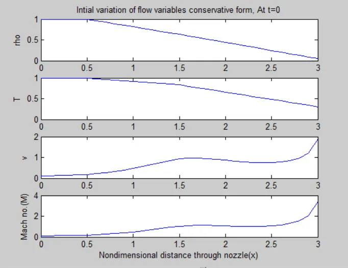
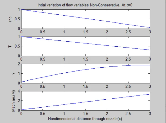
2) Variation of Mass flow rate distribution inside the nozzle at different time steps during the time-marching process
conservation form
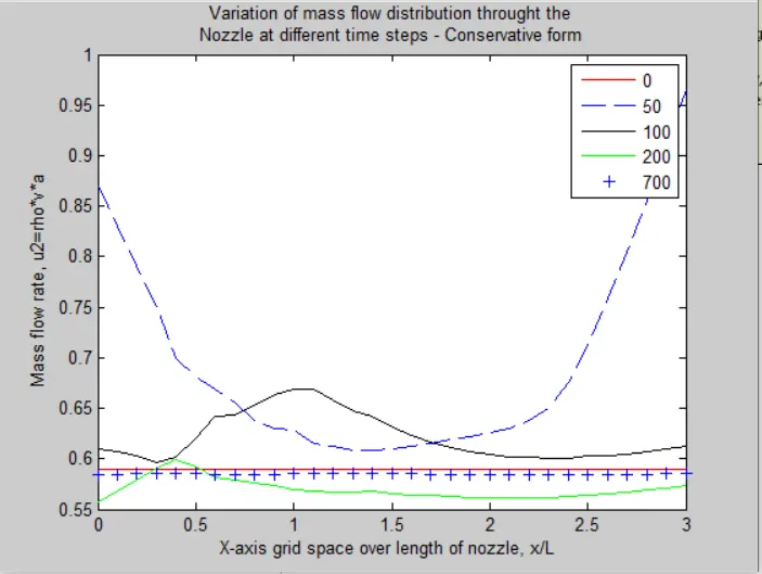
- Note that the transient mass flow deviates away from initial condition (0nt) after 100nt and after 200nt it is becoming more constant and at 700nt almost equal to constant steady state value.
Non-conservation form
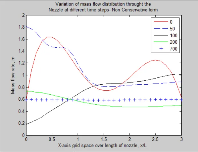
- Note that after 50nt the mass flow distribution has changed consideberly and after 100nt changed radically . however, after 200nt it is begining to settle down and after 700nt it is straight , horizontal attained steady state value.
3)Steady-state distribution of primitive variables inside the nozzle
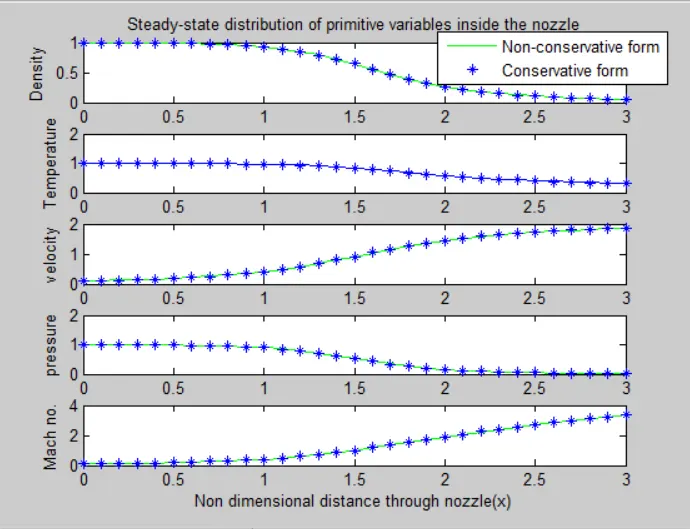
- above plot shows the steady state of both the forms.
4) Time-wise variation of the primitive variables
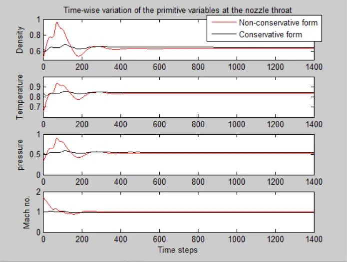
- Above plot shows the variation of p,T,rho & M at nozzle throat plotted versus no. of time steps. Note here the largest changes takes place at early times, after which the final,steady state value is approached almost asymptotically.
5)Comparison of Normalized mass flow rate distributions of both forms
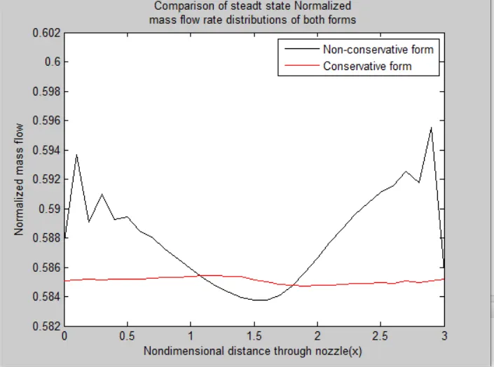
- Here we see that setady state distribution of mass flow distribution predicted by conservation form is much more satisfactory than non-conservation form solution.
6) performing grid independence test on the solution
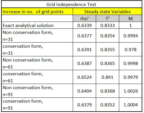
- The establised numerical solution has achived the grid inpendence, where the solution remained same for 2*N,3*N increased grid points.
- Also, we can note that Non-conservative form values are much closer to exact soln. values compared to conservative form.