Week 9 - FVM Literature Review

In CFD there are three commonly used numerical method based soolvers to solve the governing equations i.e.; Navier Stokes Equations.

These 3 methods are:

Finite Element Method (FEM):

The FEM is a particular numerical method for solving PDEs in two or three space variables. For solving a problem, the FEM subdivides a large system into smaller, simpler parts that are called Fnite Elements. The FEM finally results in a system of alzebric equations. This method approximates the unknown function over the domain. The simple equations that model these finite elements are then assembled into a larger system of equations that models the entire problem.

Finite Volume Method(FVM):

The finite volume method (FVM) is a method for representing and evaluating PDEs in the form of algebraic equations. In the finite volume method, volume integrals in a partial differential equation that contain a divergence term are converted to surface integrals, using the divergence theorem. These terms are then evaluated as fluxes at the surfaces of each finite volume. Because the flux entering a given volume is identical to that leaving the adjacent volume, these methods are conservative. Another advantage of the finite volume method is that it is easily formulated to allow for unstructured meshes. The method is used in many CFD packages. "Finite volume" refers to the small volume surrounding each node point on a mesh.

Finite Volume Method is applied over a volume so that the governing equation is valied over the entire volume. The properties are assumed to be concentrated at the centre area. The volume integrals in a partial differential equation containing a divergence term are converted into surfece integrals, using the divergence theorem. The obtained terms are considered as fluxes at the surfaces of each finite volume because when we look through these discretised equations the flux entering a given volume is considered as fluxes at the leaving the adjacent volume, which is known as conservative. FVM is widely used as it can be applied for complex geometry and moving parts.

Finite Difference Method (FDM):

Finite difference methods are discritizations used for solving differential equations by approximating them with difference equations that finite differences approximate the derivatives.

FDMs convert a linear ordinary differential equations (ODE) or non-linear partial differential equations (PDE) into a system of equations that can be solved by Matrix alzebra techniques. Foe FDMs the grid is linear and should be aligned in such a way that all grid points lie in a strite line. The properties and governing equations are considered to be concentrated at a single point.

Drawbacks of FDM:

• We cannot use FEM directly to a body whose grid points are not aligned correctly along the x,y or z directions. These situations may occur due to complex designs, folds and cuts in an geometry.
• Since it is not aligned we cannot calculate the properties at the next adjacent point exactly (since there is an inclination b/w 2 mesh points), but we can use some correction factor in order to approximate the difference with that adjacent point. This method is known as Variable Transformation Method. This approach seeks to create a grid using other space variables such as eta and epsilon. These space grids looks simlilar to a cartesian grid. A sutable mapping function is defined and this function can be easily transformed through cartician to new space variables (eta,epsilon) and vice-versa.
• The Variable Transformation Method gives an approximate solution of the property and also time consuming and complex.
• For complex profiles and moving parts the above method is less preferred.

Due to this FVM is used,

In FVM instead of writing equation for a single point, we write equations for an entire volume. Also for a considered volume no assumptions are made over the shape of the volume. Inside this particular valume the flow is conserved, flow is with 'Integral form of governing equations'.

Steps for FVM discreatisation:

1. Will write the required governing equation in its integral form.
2. Apply Gauss Divergence Theorem.
3. we Obtain discretised form which can be solved using a computer ("Flux Terms").

Consider a steady state heat conduction equation with a source term (heat generation source):

`del/(delx)(alpha*(delT)/(delx))+S=0`

Where `S` is the source term

`alpha`is thermal diffusivity term

`(delT)/(delx)` is Temperature gradient along 'x' direction.

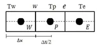
The above governing equation is valied at every point in the domain, meaning it is valied for the entire control volume. If we consider a small control volume (dv) and it is multiplied with the governing equation and integrated for entire volume then that should also be equal to zero i.e.; the integral form of the governing equation.

Taking the conservation equation validated at single point and then it is validated at entire volume and in this entire volume the properties are conserved.

Multiplying the equation by 'dv' and integrating it, we obtain

`int (del/(delx)(alpha*(delT)/(delx))+S)dv=0`

`int del/(delx)(alpha*(delT)/(delx))dv+intSdv=0`

`because dv =A.dx`

`int del/(delx)(alpha*(delT)/(delx))A*dv+intSdv=0`

`[alphaA((delT)/(delx))]_w^e+barSdv=0`

Where `barS`is the average value of source term (`S`) when multiplied by 'dv' will be equal to `intSdv`.

`alpha_eA(delT)/(delx_e)-alpha_wA(delT)/(delx_w)+barSdv=0`

if we assume `alpha` as a constant and not as a function of temperature.

`alphaA[(T_e-T_p)/(Deltax)]-alpha_wA[(T_p-T_w)/(Deltax)]+barSdv=0`

`[Heat flux]_(out) - [Heat flux]_(i) + Source term =0`

The source term which is to be added in a cell, if it is a function of temperature we have to linearize it. If we consider `alpha` as a function of temperature we have to linearize it as well.

`barS`linearization `rightarrow S_u +S_pT_p`

The amount of heat that is removed from a particular box is conserved.

Different schemes used to solve the equation:

• Gradient Scheme:

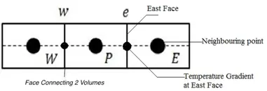
From the above figure when we calculate temperature gradient on the east face, we basically use temperature from neighbouring point trying to evaluate or numerically represent gradient of temperature which is called as gradient scheme.

• Interpolation scheme:

In the finite volume formulation, eveluation of surface and volume integrals sometimes requires the values of unknown variables at locations other than the computational nodes of the control volume. These values are obtained by employing certain interpolation schemes.

As an exmple let us consider the simple case of steady state 1D convection and diffusion.

`d/(dx)(rho u phi)=d/(dx)(Gamma(d phi)/dx)`

Where `phi` is the sloution variable (scalar)

`rho` is the density

`u` is the velocity

`Gamma` is the diffusion coeffiient.

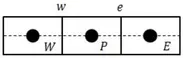
The above figure represens the three neighbouring control volumes. which we are going to use for derivating the discretization equation. Integration of the governing differential equation over the control volume around grid point P yeilds.