Week 8 - Simulation of a backward facing step in OpenFOAM
AIM:- To simulate an incompressible-laminar-viscous flow through the backward-facing step geometry in OpenFoam.
Objective:-
- To do Transient Simulation for an incompressible-laminar-viscous flow through the backward-facing step geometry
- Perform 2 case studies as described below and compare the results.
Case 1 - Simulate the flow without using any grading factor (i.e., GF = 1)
Case 2 - Simulate the flow with a grading factor of 0.2. The cells should be finer near the walls (including the step wall).
- To understand why the Grading/Growth factor is essential for meshing.
Introduction-
Backward-facing step - The study of fluid motion across various geometries is one of the major aspects of a CFD engineer. The fluid flowing over different geometries results in different flow fields (velocity field, pressure field, and more). By using this flow field data product manipulations are done for higher efficacy. In this case, a backward-facing step is used as a geometry through which fluid will be analyzed. The flow over backward-facing-step is one of the contemporary cases through which various fluid flow characteristics can be studied.
Assumptions
- The fluid flowing is a Newtonian fluid.
- The flow is incompressible and laminar.
- The kinematic viscosity is taken at the air at `T = 20^circ c`, `v = 1.516e^(-5)(m^2)/s` (Source: Air standard table)
- Zero frictional losses along with the domain.
- The backward-facing step is to be analyzed in 2-D(x and y) and we will assign negligible value to the z-direction.
Mesh specification
- Number of cells along the x-direction (longer dimension) = 200
- Number of cells along with the longer y-direction = 20;
Geometry Creation-
To create the geometry as shown in the figure, we need to edit the blockMeshDict file that is available in the system folder of the case setup
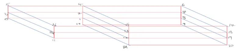
Let us consider creating the geometry using 5 blocks as shown in the figure below,
The above geometry has to be discretized into a set of blocks and combined together to create a rigid domain. So now we will discretize the domain into a set of 5 blocks.
Steps to follow - Launch OpenFoam in the Linux operating system.
Use the below shortcut commands to reach the appropriate folder to set up the files for the simulation
'ls' - to show a list of all files stored in the directories.
'cd' - To change directory
'cd ..' - To go back in the previous directory.
'pwd'- Present working directory.
'mkdir' - To create a directory.
'gedit' - used to open text editors
'cp -r' - To copy folder
'rm' - to remove files
'rm -r' - to remove/delete directories
'tut' - shortcut to open tutorials folder of OpenFOAM
'app' - applications
'sol' - solvers
'$FOAM_RUN' - navigates to OpenFOAM run directory
'paraFoam' - opens paraView(data analysis and visualization application) where the simulation is represented
- Now, by using the above commands of OpenFOAM we reach the cavity folder
tutorial `implies` incompressible `implies` icoFoam `implies` cavity
- Again type (cp -r cavity/ $FOAM_RUN/ test)
Here cp is the syntax used to copy any file or folder, "-r" is used to denote the entire directory with all the files then "$FOAM_RUN" is the run directory inside the OpenFOAM which allows the user to run user modified problems or tutorials.
this will create a new folder named 'test' and paste the cavity folder into it.
- Now, we are going to edit the scripts files in the cavity directory. Here we are having various directories with different significance.
blockMeshDict (test/cavity/cavity/system/blockMeshDict): It has the geometric and mesh characteristics of the domain.
transportProperties (test/cavity/cavity/constant/transportProperties): It has the information of the transport quantity. In our case, the transport object is air and the transport property is kinematic viscosity (νν).
controlDict (test/cavity/cavity/system/controlDict): It has the time control (features like start time, end time, deltaT, writeControl, writeInterval and many more). It governs the time adjustments and modifications.
fvSchemes (test/cavity/cavity/system/fvSchemes): It sets the numerical schemes for terms such as derivatives in equations that are calculated in the simulation. It has the categories such as gradient, divergence, Laplacian, time derivatives, etc.
fvSolution (test/cavity/cavity/system/fvSolution): It governs the equations, solvers and numerical algorithm.
So the above files need to be modified as per our requirement for our project
Step 1- Editing the blockMeshDict file
Here, in this script file, we will edit the vertices of the geometry, also as our geometry is in centimeters(cm), we will use the conversion criteria for it to convert it into meters(m)
/*--------------------------------*- C++ -*----------------------------------*\
  =========                 |
  \\      /  F ield         | OpenFOAM: The Open Source CFD Toolbox
   \\    /   O peration     | Website:  https://openfoam.org
    \\  /    A nd           | Version:  8
     \\/     M anipulation  |
\*---------------------------------------------------------------------------*/
FoamFile
{
    version     2.0;
    format      ascii;
    class       dictionary;
    object      blockMeshDict;
}
// * * * * * * * * * * * * * * * * * * * * * * * * * * * * * * * * * * * * * //

convertToMeters 0.01;

vertices
(
    (0 0 0)    // vertex 0
    (0 0 1)    // vertex 1
    (8 0 1)    // vertex 2
    (8 0 0)    // vertex 3
    (0 0.5 0)  // vertex 4
    (0 0.5 1)  // vertex 5
    (8 0.5 1)  // vertex 6
    (8 0.5 0)  // vertex 7
    (0 1 0)    // vertex 8
    (0 1 1)    // vertex 9
    (8 1 1)    // vertex 10
    (8 1 0)    // vertex 11
    (8 -1 1)   // vertex 12
    (20 -1 1)  // vertex 13
    (20 -1 0)  // vertex 14
    (8 -1 0)   // vertex 15
    (20 0 1)   // vertex 16
    (20 0 0)   // vertex 17
    (20 0.5 1) // vertex 18
    (20 0.5 0) // vertex 19
    (20 1 1)   // vertex 20
    (20 1 0)   // vertex 21
);

blocks
(
    hex (0 3 7 4 1 2 6 5) (50 10 1) simpleGrading (1 5 1)
    hex (4 7 11 8 5 6 10 9) (50 10 1) simpleGrading (1 0.2 1)
    hex (15 14 17 3 12 13 16 2) (150 20 1) simpleGrading (5 10 1)
    hex (3 17 19 7 2 16 18 6) (150 10 1) simpleGrading (5 5 1)
    hex (7 19 21 11 6 18 20 10) (150 10  1) simpleGrading (5 0.2 1)
);

edges
(
);

boundary
(
    inlet
    {
        type patch;
        faces
        (
            (0 1 5 4)
            (4 5 9 8)
        );
    }
    outlet
    {
        type patch;
        faces
        (
            (14 17 16 13)
            (17 19 18 16)
            (19 21 20 18)
        );
    }
    walls
    {
        type wall;
        faces
        (
            (8 9 10 11)
            (0 3 2 1)
            (11 10 20 21)
            (15 14 13 12)
            (15 12 2 3)
        );
     }
    frontAndBack
    {
        type empty;
        faces
        (
            (1 5 6 2)
            (5 9 10 6)
            (12 2 16 13)
            (2 6 18 16)
            (6 10 20 18)
            (0 3 7 4)
            (4 7 11 8)
            (15 14 17 3)
            (3 17 19 7)
            (7 19 21 11)
        );
    }
);

mergePatchPairs
(
);

// ************************************************************************* //
- In blockMeshDict file as the Geometry is backward facing step. we will discretize it into 5 blocks and index the vertices
- Then we will combine all the individual blocks with the appropriate vertices to another block.
- The starting letter "hex" defines the "hexahedral" type of mesh for the block meshing.
Case-1 - The total number of cells along the x-direction is given to be as 200 and for y-direction, it is given as 20. And here simple grading of (1 1 1) is used, which means the cells along the three dimensions are equally spaced (uniform).
Case -2 - As the grading factor helps to stretch the mesh along one direction. The mesh grading is given to capture the physics at a particular area. For our purpose, grading is required at the step wall, bottom wall, top wall, and the no-slip wall. As more of physics is concerned at this locations.
Mesh grading is given as a factor of 5, 10, 0.2 which same but changes as per the orientation of the domain (i.e position of starting and ending cell).
Boundary condition
- There are various boundaries in our domain which are inlet, outlet, front & back, and no-slip wall (velocity of the immediate fluid layer along the wall surface tends to be zero).
- For Inlet and Outlet face from where fluid enters and exits 'patch' type boundary is used. In OpenFOAM 'patch' is refereed as the condition that contains no geometric or topological information about the mesh(with the exception of the wall)
- The front and back boundary faces are provided since we are not interested in the 3D analysis of the backward-facing step. considered as no flow in that direction
- The top, bottom, and step face is referred to be as "no-slip wall", where boundary condition of "wall" is assigned. OpenFOAM will treat as a wall with a no-slip phenomenon at its surface.
Step 2- Editing the controlDict file
- The controlDict script file controls the time functions such as startTime stopTime, deltaT, writeControl, etc.
- startTime and endTime value is provided s 0 and 20.
- So time step modification is done by taking time step as 1e-3 (as it affects the CFL criterion). Such time step should be rationally guessed or one may try with some initial guess and according to expected CFL, if not satisfied or error occurs then may decrease it accordingly.
/*--------------------------------*- C++ -*----------------------------------*\
  =========                 |
  \\      /  F ield         | OpenFOAM: The Open Source CFD Toolbox
   \\    /   O peration     | Website:  https://openfoam.org
    \\  /    A nd           | Version:  8
     \\/     M anipulation  |
\*---------------------------------------------------------------------------*/
FoamFile
{
    version     2.0;
    format      ascii;
    class       dictionary;
    location    "system";
    object      controlDict;
}
// * * * * * * * * * * * * * * * * * * * * * * * * * * * * * * * * * * * * * //

application     icoFoam;

startFrom       startTime;

startTime       0;

stopAt          endTime;

endTime         20;

deltaT          1e-3;

writeControl    timeStep;

writeInterval   20;

purgeWrite      0;

writeFormat     ascii;

writePrecision  6;

writeCompression off;

timeFormat      general;

timePrecision   6;

runTimeModifiable true;


// ************************************************************************* //
Step -3 Edit the transportProperty file
In this directory we will edit the kinematic viscosity of to `1.516e^(-5) m^2/s` from the initial value. As we are assuming air to be at `T = 20^circ` C,
/*--------------------------------*- C++ -*----------------------------------*\
  =========                 |
  \\      /  F ield         | OpenFOAM: The Open Source CFD Toolbox
   \\    /   O peration     | Website:  https://openfoam.org
    \\  /    A nd           | Version:  8
     \\/     M anipulation  |
\*---------------------------------------------------------------------------*/
FoamFile
{
    version     2.0;
    format      ascii;
    class       dictionary;
    location    "constant";
    object      transportProperties;
}
// * * * * * * * * * * * * * * * * * * * * * * * * * * * * * * * * * * * * * //

nu              [0 2 -1 0 0 0 0] 1e-5;


// ************************************************************************* //
Step 4 - Then we reach the '0' directory(test/cavity/cavity/0) to edit the Velocity and Pressure files as per our requirement
Edit the pressure(p) file
- Pressure at inlet is stated to be as zeroGradient (Neumann B.C.) and outlet pressure is explicitly stated as "uniform 0" (at 1 atm) (Dirichlet B.C.).
- Front and back patches are kept empty (AS no velocity field is calculated at this patch).
- And for the no-slip wall boundary, pressure is defined to be as zeroGradient(Neumann B.C.)
/*--------------------------------*- C++ -*----------------------------------*\
  =========                 |
  \\      /  F ield         | OpenFOAM: The Open Source CFD Toolbox
   \\    /   O peration     | Website:  https://openfoam.org
    \\  /    A nd           | Version:  8
     \\/     M anipulation  |
\*---------------------------------------------------------------------------*/
FoamFile
{
    version     2.0;
    format      ascii;
    class       volScalarField;
    object      p;
}
// * * * * * * * * * * * * * * * * * * * * * * * * * * * * * * * * * * * * * //

dimensions      [0 2 -2 0 0 0 0];

internalField   uniform 0;

boundaryField
{
    inlet
    {
        type            zeroGradient;
    }

    outlet
    {
        type            fixedValue;
        value           uniform 0;
    }

    walls
    {
        type            zeroGradient;
    }

    frontAndBack
    {
        type            empty;
    }
}
// ************************************************************************* //
Step 5 - Edit the velocity(U) file
- We assume uniform velocity at the inlet condition as U = (0.02 0 0) (U = 0.02 m/sec in x-direction and U=0 in y-z direction) (Dirichlet boundary condition).
- Outlet will be kept as zeroGradient at the initial state but will be calculated as a function of time step advancement (Neumann boundary condition).
- walls at "noSlip" boundary condition
/*--------------------------------*- C++ -*----------------------------------*\
  =========                 |
  \\      /  F ield         | OpenFOAM: The Open Source CFD Toolbox
   \\    /   O peration     | Website:  https://openfoam.org
    \\  /    A nd           | Version:  8
     \\/     M anipulation  |
\*---------------------------------------------------------------------------*/
FoamFile
{
    version     2.0;
    format      ascii;
    class       volVectorField;
    object      U;
}
// * * * * * * * * * * * * * * * * * * * * * * * * * * * * * * * * * * * * * //

dimensions      [0 1 -1 0 0 0 0];

internalField   uniform (0 0 0);

boundaryField
{
    inlet
    {
        type            fixedValue;
        value           uniform (0.02 0 0);
    }

    outlet
    {
        type            zeroGradient;
    }

    walls
    {
        type            noSlip;
    }
}

// ************************************************************************* //
Visualization of the meshing in paraView
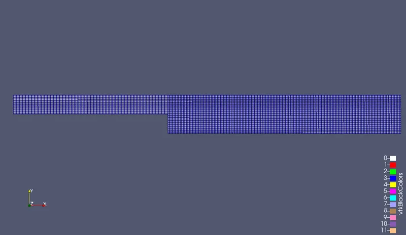
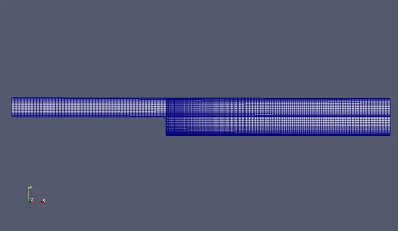
Graded mesh can be visualized in the Paraview interface, the finer mesh can be seen at the step wall and at the top and bottom wall, as these are the location where more physics must get captured.
Case-1
Creating a Mesh for Grading Factor = 1
- In this case, the grading factor is kept as 1 for all x,y, z-direction
- Now we use 'icoFoam' command in the script terminal to solve our problem, and if there were no errors found we will run the paraView to proceed with the simulation.
- Now, after opening the paraView visualization app, we tap 'apply' at the left of the interface of the application to visualize the mesh geometry.
- Now select the surface with edges and velocity(U) to visualize the geometry ready for execution.
- Finally, start the simulation to visualize results by clicking on the start button.
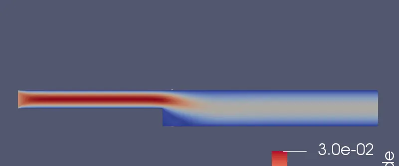
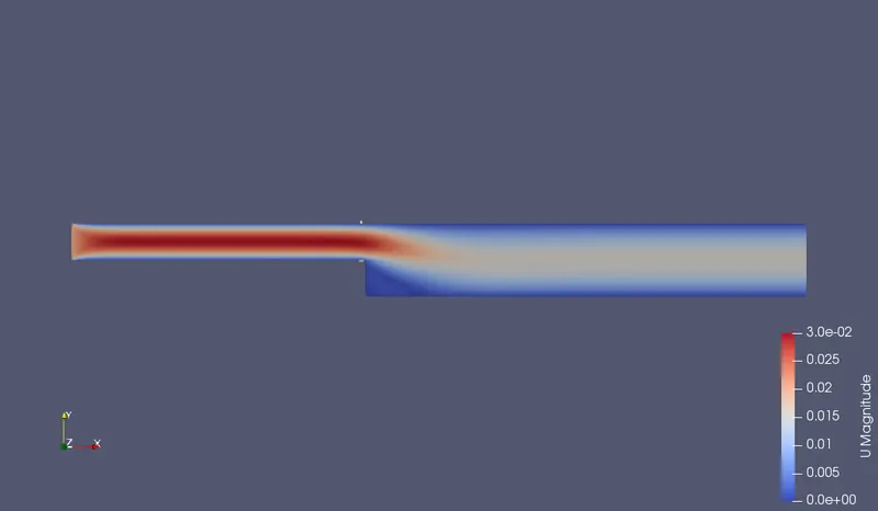
Velocity contour result- The velocity contour plot results show the velocity distribution, flow separation, boundary layer formation, free-stream velocities, recirculation zone, and much more physics.
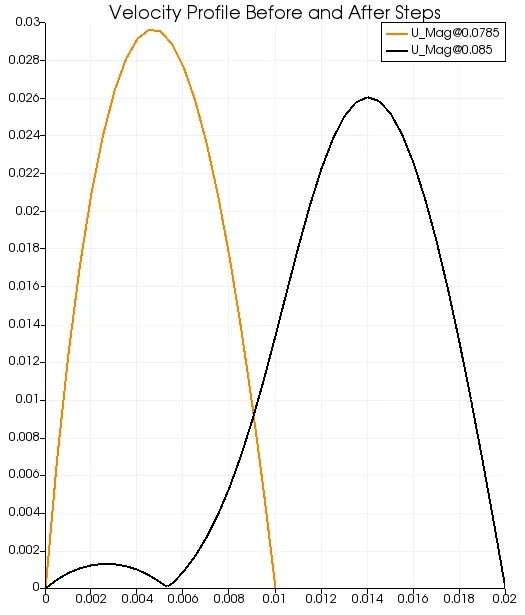
Compare the Velocity Profiles before and after the step
- We can compare the velocity profile just before the step is started with a point just after the step.
- Below are the comparison of the profiles at the points 0.078 and 0.085 in the x-direction
Case-2
- In this case, the grading factor is kept as 0.2.
- Now repeat the process as done in case 1 to run the simulation.
- Finally, start the simulation to visualize results by clicking on the start button.
Creating a Mesh for Grading Factor = 0.2
Velocity contour result- The velocity contour plot results show the velocity distribution, flow separation, boundary layer formation, free-stream velocities, recirculation zone, and much more physics.
Compare the Velocity Profiles before and after the step-
- We can compare the velocity profile just before the step is started with a point just after the step.
- Below are the comparison of the profiles at the points 0.078 and 0.085 in the x-direction
- As it is shown from the graph that the magnitude of velocity suddenly decreases as the area is increases
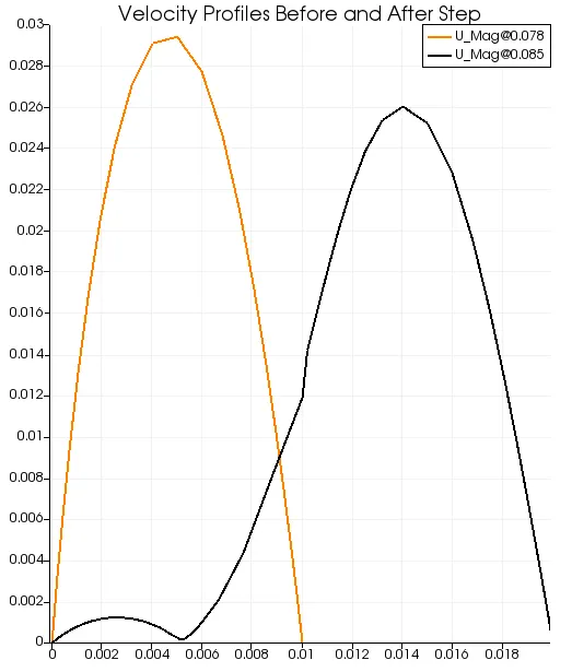
Result explanation after simulation for both cases (velocity before and after step)
- When the fluid crosses the step region the area increases and velocity reduces and then velocity takes the constant profile along the duct
- The sudden enlargement in the cross-section breaks the boundary layer at the step corner. The significance of wall shear stress gets zero. The velocity of the fluid layer adjacent to the wall surface stays no longer zero. It has to change as its contact with the wall surface is disturbed.
Now, the velocity of the bottommost fluid layer has two choices:
1) To move further along with the flow in positive x-direction or
2) To flow in the negative x-direction.
Here at this condition, the bottommost fluid layer will try to flow in the negative x-direction. This is because of some unusual phenomenon called the adverse pressure gradient
- In fluid dynamics, an adverse pressure gradient occurs when the static pressure increases in the direction of the flow. This is important for boundary layers.
Increasing the fluid pressure is akin to increasing the potential energy of the fluid, leading to reduced kinetic energy and deceleration of the fluid. Since the fluid in the inner part of the boundary layer is slower, it is more greatly affected by the increasing pressure gradient. For a large enough pressure increase, this fluid may slow to zero velocity or even become reversed causing a flow separation. This has very significant consequences in aerodynamics since flow separation significantly modifies the pressure distribution along the surface and hence the lift and drag characteristics.
Comparison of both the cases1,2 on the basis of grading factor: Why Grading/Growth factor is essential for meshing.
On comparing the velocity profile for both cases.
- As we know that, the more the finer mesh, the more is the accurate result (least residuals in the approximation).
The velocity profile after the step is measured in both the cases, however in both cases velocity profiles looks almost similar but case 2 (with grading) produced more accurate results than that of case1 (no grading).
- Let's have a look at the velocity profile measured along with y distance at x = 0.085m. Additionally, if the mesh is not fine enough at the location where is fluid behavior is more of concern, it will give average results because it has fewer elements to capture the physics at each node or at each element volume. So in order to get the most accurate results, it is required to have a sufficiently finer mesh size to capture the flow properties of the fluid.
- By comparing we have an intuition that mesh size or cell size will have significant consequences on our results. At x = 0.085, the incoming fluid passed the way of boundary layer separation. So from the bottom of the enlarged s/c (0.085,0) to (0.085,0.02), velocity will increase in the y-dimension. However, after undergoing flow separation, the velocity increment in the y-direction won't be uniform, it should have patterns of variations along the y-direction. The velocity is recirculating in this section after flow separation, hence it cannot have a uniform increment in the y-direction.
Moreover, the velocity distribution at the top wall must show variation in velocity because of the presence of the boundary layer, and appropriate velocity distribution is shown by case 2.
Since the velocity distribution shown resulted by case 2 at x = 0.085m shows more accurate results than that of case 1.
- We can call this study a grid dependency test, as the flow field variables change significantly as a function of the mesh or grid size.
Conclusion:-
- When the fluid crosses the step region the area increases and velocity reduces and then velocity takes the constant profile along the duct.
- There is no significant effect in simulation because of the change in grading factor, and also there is no significant effect in velocity profile there is a minor difference in maximum and minimum value.
- Overall the grading schemes gives us the same results, but due to the mesh grading factor we can say that velocity gradient of 0.2 shows more accurate results as compared to the GF = 1