Week 8 - Simulation of a backward facing step in OpenFOAM
AIM: To simulate an incompressible-laminar-viscous flow through the backward facing step geometry and should perform a transient simulation using multiple meshes refining mesh grading factors inside blockMeshDict file of blockMesh using openfom with the help of icoFoam solver.
Mesh specifications:
- Number of cells along the x direction (longer dimension) = 200
- Number of cells along the longer y direction = 20
- Use graded mesh on which you will perform 2 case studies as described below and also compare the results i.e,
- Simulate the flow without using any grading factor (i.e., GF = 1)
- Simulate the flow with grading factor of 0.2. The cells should be finer near the walls (includig the step wall).
Theory:-
OpenFOAM ("Open-source Field Operation And Manipulation") is a C++ toolbox for the development of customized numerical solvers, and pre-/post-processing utilities for the solution of continum mechanics problems, most prominently including computational fluid mechanics (CFD).
OpenFOAM is the free, open source CFD software developed primarily by OpenCFD Ltd since 2004. It has a large user base across most areas of engineering and science, from both commercial and academic organisations. OpenFOAM has an extensive range of features to solve anything from complex fluid flows involving chemical reactions, turbulence and heat transfer, to acoustics, solid mechanics and electromagnetics.
Boundary layer Theory:-
Boundary layer, in fluid mechanics, thin layer of a flowing gas or liquid in contact with a surface such as that of an airplane wing or of the inside of a pipe. The fluid in the boundary layer is subjected to shearing forces. A range of velocities exists across the boundary layer from maximum to zero, provided the fluid is in contact with the surface. Boundary layers are thinner at the leading edge of an aircraft wing and thicker toward the trailing edge. The flow in such boundary layers is generally laminar at the leading or upstream portion and turbulent in the trailing or downstream portion.
Boundary layer seperation over a flat plate:-
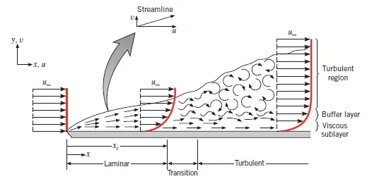
- It is the locus of the point at which the velocity of fluid becomes equal to 99% of the free steam velocity i.e, (u0 or u-infinity).
- The free stream flow which has uniform velocity u0 when passes over a solid surface there is zero velocity (no slip) at the solid surface and gradually increases upto 99% of free stream velocity normal to the flow direction.
- Within the boundary layer fluid is viscous and velocity gradient i.e,(dy/dx) setup thats why the shear stress are present the flow will be rotational in nature.
- beyond the boundary layer the fluid is viscous but there is no velocity gradient that's why shear stress = 0 and it behave like a ideal flow.
- Some distance from the leading edge the bounday layer is laminar in nature and velocity profile is parabolic in character.
- After a certain point there is transition zone in which the flow is becomes unstable and after a particular distance it switch to turbulent flow boundary layer here the velocity profile is parabolic in nature but the turbulent flow boundary layer is logrithmic in character.
Operating system and Interface of OpenFoam:-
Operating system here we are using linux on Ubuntu. Hence it is command line Interface (CLI), It uses text based Interface (UI) to view and manage computer files.
Short commands that we are using this project:-
- ls - list of all files that stored in the directories.
- cd - To change directory
- cd .. - To go back in the previous directory.
- pwd - Present working directory.
- mkdir - To create directory.
- cp - To copy
- tut - tutorials of openfoam
- app - applications
- rm - to remove files
- rm -r - to remove directories
- gedit - used to open text editors
- sol - solvers
- $FOAM_RUN - navigates to openfoam run directory
- paraFoam - opens paraview where the simulation is represented.
Steps to be done in this project of Openfoam:-
- Choosing a solver from the tutorials
- Creating a Geometry
- Editing blockMishDict file
a) Boundary conditions.
b)Initial conditions.
- Pressure
- Velocity
- Editing ControlDict file
- Velocity profile and line plots for before and after the step facing
- Comparsion of both the plots for velocity profile
- we can also solve for grading factor = 1 and see the difference between the GF = 1 and GF = 0.2
- Conclusion
Explanation of the project that is made by using openFoam:-
- First we launch the Ubuntu and Open the terminal in the OS
- we are using the linux or command line interface to run the openFoam
- After that First we have to type the openFoam shortcut command 'tut' for openFoam tutorials It goes to directly in the tutorials folder
- Then we use cd command to change the directory and goes into the new directory So, type cd with the name of folder which we are going to open. In this case we are going to open the incompressible directory.
- Then check the files stored in the incompressible file type ls command and copy the cavity folder to $FOAM_RUN using with the command cp -r cavity/$FOAM_RUN.
- $FOAM_RUN use the openfoam shortcut 'run'
- Then we are going to use cd cavity command to go inside the cavity folder and inside the cavity we got 3 files named as 0 constant system
- Inside the system folder we have blockMeshDict file, controlDict file, boundary conditions file, fvSchemes, and fvSolutions. blockMeshDict file and controlDict files needs to be edit which we are going to edit in the text Form which we have to edited.
- After editing the blockMeshDict file and controlDict file according to the needs of the questions or projects we are going next to edit the intial conditions file.
- Now we are going inside the 0 folder in this we have the initial conditions like Pressure and velocity, Now we have to edit this conditions also as per requirements.
- Now return back to the cavity folder by using cd ../ command and blockMesh command is used to creates the Mesh and other Calculations are done.
- Now, type icoFoam to calculate the simulation and after once simulations timing and other caculations are done
- Type paraFoam command to open paraview for post processing
- When paraview is open click on apply after selecting the fields like Velocity and presssure.
- After that you can simulate the data by clicking on the simulation with respect of time and see the simulation takes place and also check how the velocity profile takes place.
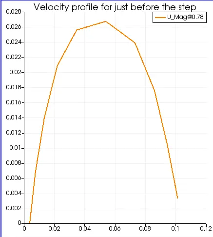
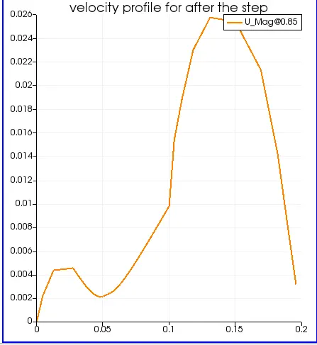
- After that you can plot the data by click on the plot over line command and pointing out the line on that axis or place where you can check the velocity change. In this case we are checking the velocity profile after and before the step .
- after this we have save the screenshots and plots of this data by clicking on the save screenshots in file folder.
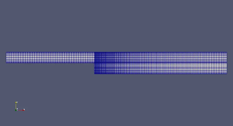
Creating a Geometry-The domain specifications are provided in the following figure and to create the geometry we need to edit the blockMeshdict file that is available in the system folder of the case setup.
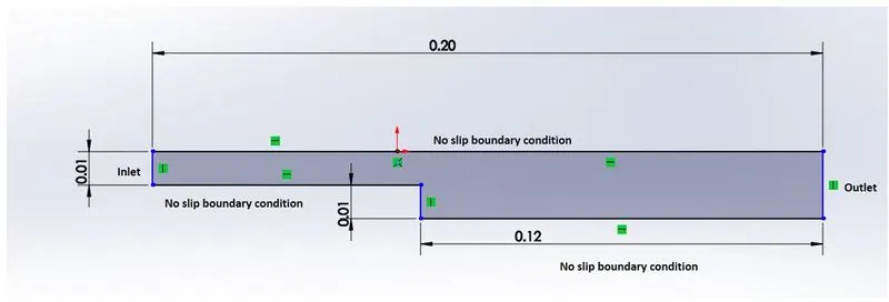
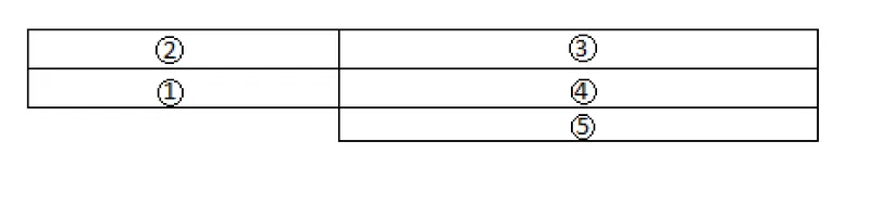
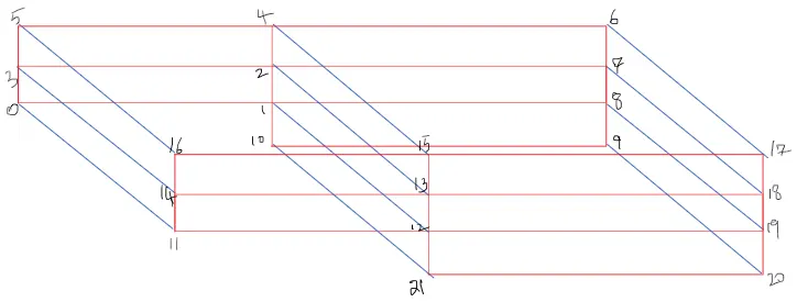
We are going to edit the blockMeshDict file to create the given Geometry using backward facing step. Hence it can only be done in blocks, we have considered it as 5 blocks and indexed the vertices as shown in figure.
- Editing the blockMeshDict file:-
/*--------------------------------*- C++ -*----------------------------------*\
  =========                 |
  \\      /  F ield         | OpenFOAM: The Open Source CFD Toolbox
   \\    /   O peration     | Website:  https://openfoam.org
    \\  /    A nd           | Version:  8
     \\/     M anipulation  |
\*---------------------------------------------------------------------------*/
FoamFile
{
    version     2.0;
    format      ascii;
    class       dictionary;
    object      blockMeshDict;
}
// * * * * * * * * * * * * * * * * * * * * * * * * * * * * * * * * * * * * * //

convertToMeters 0.1;

vertices
(
    (0 0 0) //vertex 0
    (8 0 0) //vertex 1
    (8 0.5 0) //vertex 2
    (0 0.5 0) //vertex 3
    (8 1 0) //vertex 4
    (0 1 0) //vertex 5
    (20 1 0) //vertex 6
    (20 0.5 0) //vertex 7
    (20 0 0) //vertex 8
    (20 -1 0) //vertex 9
    (8 -1 0) //vertex 10
    (0 0 1) //vertex 11
    (8 0 1) //vertex 12
    (8 0.5 1) //vertex 13
    (0 0.5 1) //vertex 14
    (8 1 1) //vertex 15
    (0 1 1) //vertex 16
    (20 1 1) //vertex 17
    (20 0.5 1) //vertex 18
    (20 0 1) //vertex 19
    (20 -1 1) //vertex 20
    (8 -1 1) //vertex 21

);

blocks
(
    hex (0 1 2 3 11 12 13 14) (50 5 1) simpleGrading (1 5 1)
    hex (3 2 4 5 14 13 15 16) (50 5 1) simpleGrading (1 0.2 1)
    hex (2 7 6 4 13 18 17 15) (150 5 1) simpleGrading (5 0.2 1)
    hex (1 8 7 2 12 19 18 13) (150 5 1) simpleGrading (5 5 1)
    hex (10 9 8 1 21 20 19 12) (150 5 1) simpleGrading (5 10 1)
);

edges
(
);

boundary
(
   inlet
    {
        type patch;
        faces
        (
            (0 11 14 3)
            (3 14 16 5)
        );
    }
    outlet
    {
        type patch;
        faces
        (
            (9 8 19 20)
            (8 7 18 19)
            (7 6 17 18)
        );
    }
    walls
    {
        type wall;
        faces
        (
            (4 5 16 15)
            (6 4 15 17)
            (0 1 12 11)
            (10 9 20 21)
            (10 21 12 1)
        );
    }
);

// ************************************************************************* //
- Boundary conditions:- After defining the boundary conditions correctly check it that you have define them correctly or not then execute the blockMesh command in the terminal. Now open the parafoam, deselect the fields otherwise its not going to work because at this time we haven't edits the fields like velocity and pressure. after this you have to click on apply now you can see the Mesh.
- Initial conditions:-we have to edits this initial conditions for working out the simulations correctly.
1. Pressure file :-
/*--------------------------------*- C++ -*----------------------------------*\
  =========                 |
  \\      /  F ield         | OpenFOAM: The Open Source CFD Toolbox
   \\    /   O peration     | Website:  https://openfoam.org
    \\  /    A nd           | Version:  8
     \\/     M anipulation  |
\*---------------------------------------------------------------------------*/
FoamFile
{
    version     2.0;
    format      ascii;
    class       volScalarField;
    object      p;
}
// * * * * * * * * * * * * * * * * * * * * * * * * * * * * * * * * * * * * * //

dimensions      [0 2 -2 0 0 0 0];
 //Kinematic Pressure = P/rho

internalField   uniform 0;

boundaryField
{
    inlet
    {
        type           zeroGradient;
    }

   outlet
    {
        type            fixedValue;
        value           uniform 0;
    }

    walls
    {
        type            zeroGradient;
        }
}

// ************************************************************************* //
2. Velocity file:-
/*--------------------------------*- C++ -*----------------------------------*\
  =========                 |
  \\      /  F ield         | OpenFOAM: The Open Source CFD Toolbox
   \\    /   O peration     | Website:  https://openfoam.org
    \\  /    A nd           | Version:  8
     \\/     M anipulation  |
\*---------------------------------------------------------------------------*/
FoamFile
{
    version     2.0;
    format      ascii;
    class       volVectorField;
    object      U;
}
// * * * * * * * * * * * * * * * * * * * * * * * * * * * * * * * * * * * * * //

dimensions      [0 1 -1 0 0 0 0];

internalField   uniform (0 0 0);

boundaryField
{
 inlet
    {
        type            fixedValue;
        value           uniform (0.02 0 0);
    }

   outlet
    {
        type            zeroGradient;
    }

    walls
    {
        type            noSlip;
    }
}

// ************************************************************************* //
ControlDict file :-
/*--------------------------------*- C++ -*----------------------------------*\
  =========                 |
  \\      /  F ield         | OpenFOAM: The Open Source CFD Toolbox
   \\    /   O peration     | Website:  https://openfoam.org
    \\  /    A nd           | Version:  8
     \\/     M anipulation  |
\*---------------------------------------------------------------------------*/
FoamFile
{
    version     2.0;
    format      ascii;
    class       dictionary;
    location    "system";
    object      controlDict;
}
// * * * * * * * * * * * * * * * * * * * * * * * * * * * * * * * * * * * * * //

application     icoFoam;

startFrom       startTime;

startTime       0;

stopAt          endTime;

endTime         20;

deltaT          1e-2;

writeControl    timeStep;

writeInterval   20;

purgeWrite      0;

writeFormat     ascii;

writePrecision  6;

writeCompression off;

timeFormat      general;

timePrecision   6;

runTimeModifiable true;


// ************************************************************************* //
After this code we goes again in the terminal and type the icoFoam command to calculate the simulations and Once the simulation is done type paraFoam command to open the paraview for post processing.
When mesh Grading Factor is taken to be 0.2
    hex (0 1 2 3 11 12 13 14) (50 5 1) simpleGrading (1 5 1)
    hex (3 2 4 5 14 13 15 16) (50 5 1) simpleGrading (1 0.2 1)
    hex (2 7 6 4 13 18 17 15) (150 5 1) simpleGrading (5 0.2 1)
    hex (1 8 7 2 12 19 18 13) (150 5 1) simpleGrading (5 5 1)
    hex (10 9 8 1 21 20 19 12) (150 5 1) simpleGrading (5 10 1)
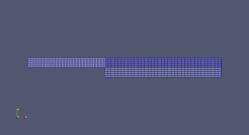
Creating a Mesh for Grading Factor = 0.2
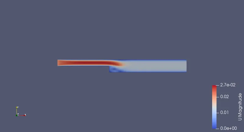
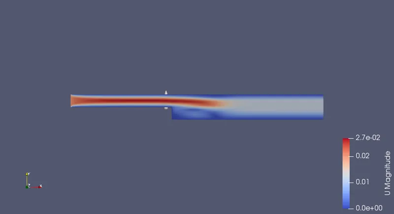
Simulation Process we can clearly see the velocity profile in this simulation and how it is changing inside the duct.
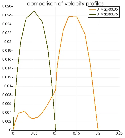
Velocity Profiles before and after the step:-
Comparison between both the plots:-
When mesh Grading Factor is taken to be 1
    hex (0 1 2 3 11 12 13 14) (50 5 1) simpleGrading (1 1 1)
    hex (3 2 4 5 14 13 15 16) (50 5 1) simpleGrading (1 1 1)
    hex (2 7 6 4 13 18 17 15) (150 5 1) simpleGrading (1 1 1)
    hex (1 8 7 2 12 19 18 13) (150 5 1) simpleGrading (1 1 1)
    hex (10 9 8 1 21 20 19 12) (150 5 1) simpleGrading (1 1 1)
Creating a Mesh for Grading Factor = 1
Simulation Process we can clearly see the velocity profile in this simulation and how it is changing inside the duct.
Velocity Profiles before and after the step:-
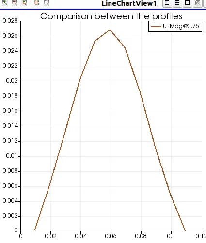
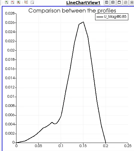
Comparison between both the plots:-
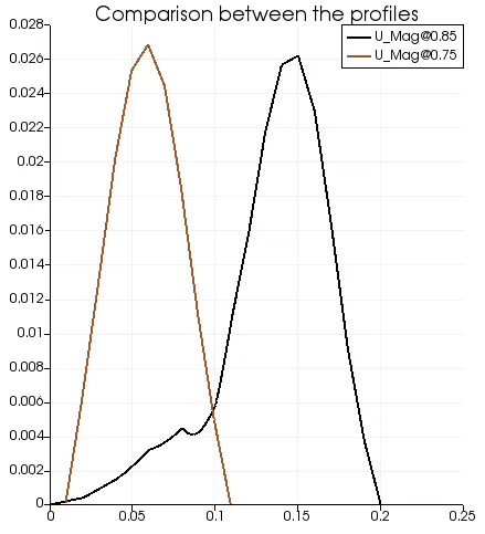
Conclusion:-
- When the fluid crosses the step region the area increses and velocity reduces and then velocity takes the constant profile along the duct.
- There is no sgnificant effect in simulation because of change in grading factor. and also there is no significant effect in velocity profile there is minor difference in maximum and minimum value.
- When the grading factor is 0.2 mesh can be easily seen as it is less congested.
- Performing a simulation is easier in case of parafoam.
- Overall the grading schemes gives us the same results, but due to the mesh grading factor we can say that velocity gradient of 0.2 shows more accurate results as compared to the GF = 1