Week 8 - Simulating Cyclone separator with Discrete Phase Modelling

 AIM:

• Perform analysis on cyclone separator using Ansys Fluent software by varying the particle diameter from 1 μm to 5 μm and calculate the separation efficiency in each case. Discuss the results. [Use both the velocity as 3m/sec.]
• Perform an analysis on a given cyclone separator model by varying the particle velocity from 1 m/sec to 5 m/sec and calculate the separation efficiency and pressure drop in each case. Discuss the results. [Use particle diameter size as 5 μm for all cases & keep flow velocity same as particle velocity]

Boundary Conditions:-

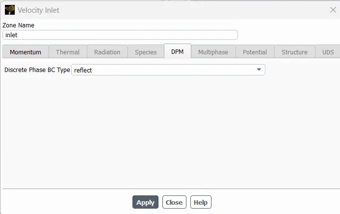
Inlet and wall: - Reflect

Outlet (Top):- Escape 

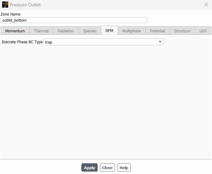
Outlet (Bottom/dustbin) - Trap

Expected results:

• Explain discrete phase modeling.
• Calculate cyclone separator efficiency for each cases.
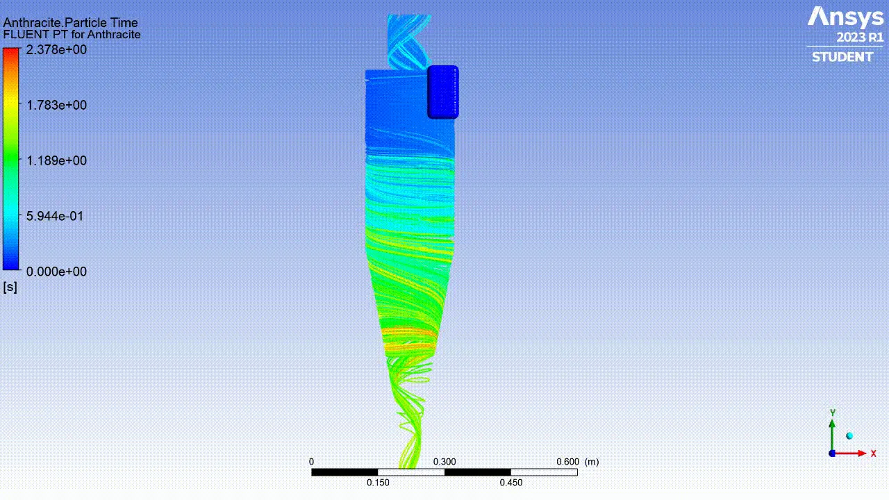
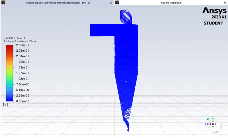
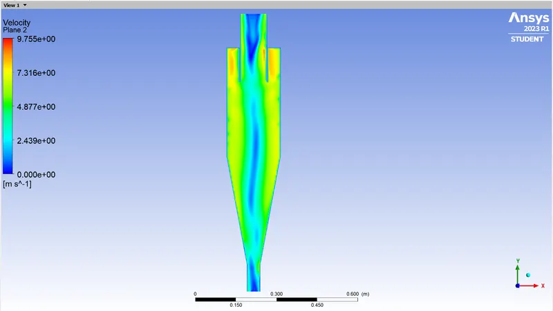
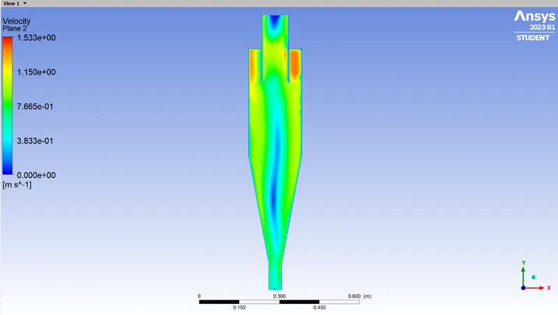
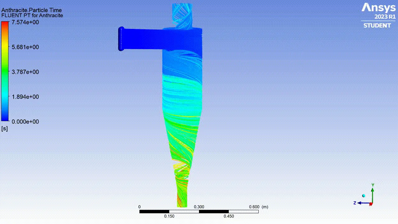
• Velocity, pressure & Particle time.

INTRODUCTION:

Cyclone separators are widely used in industries to separate particles from gas or liquid streams. The performance of a cyclone separator depends on several factors, such as the particle size, particle density, and fluid flow rate. To optimize the design and operation of cyclone separators, it is essential to have a deep understanding of the fluid-particle interaction inside the cyclone.

THEORY:

Discrete phase modeling is a computational fluid dynamics (CFD) technique used to simulate the behavior of dispersed particles or droplets in a fluid. It is used when there is a need to study the motion and interactions of a large number of particles or droplets in a fluid flow, such as in spray painting, fuel injection, or chemical reactions involving particles. In discrete phase modeling, the particles or droplets are treated as individual entities that move and interact with the surrounding fluid flow. The particles are tracked using Lagrangian methods, where each particle is represented by a discrete particle trajectory. The fluid flow is modeled using Eulerian methods, where the fluid is divided into a grid and the fluid properties are computed at each point in the grid.

The interaction between the particles and the fluid is modeled using a variety of physical models, such as drag forces, gravity, and turbulence effects. The forces acting on the particles can be calculated based on the fluid properties at the location of the particle, such as the velocity, pressure, and turbulence characteristics of the fluid flow. Discrete phase modeling can be used to predict a variety of phenomena related to dispersed particles, such as the distribution and concentration of particles in a flow, the trajectory and collision of particles, and the deposition of particles on surfaces. It can also be used to optimize the design and operation of devices that involve particle or droplet transport, such as fuel injectors or spray nozzles.

SOLVING & MODELING APPROACH:

In this simulation, Particles along with air is passed through the inlet of the cyclone separator with different inlet velocities from 1 m/sec to 5 m/sec and allowed to pass through the outlet to calculate the separation efficiency and pressure drop by using RNG k-epsilon model until the solution is converged. Different size of particles is used for the simulation. Cutshell method will be used for refined mesh. RNG k-epsilon model is used because it gives better results when there is a free flow of the fluid and in swirl formations.

PRE-PROCESSING AND SOLVER SETTING:

Geometry:

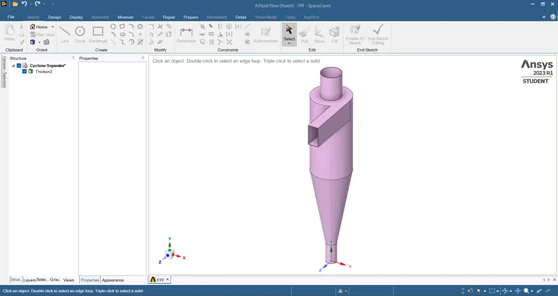
• Run ANSYS 2023 R1 student version and drag Fluid Flow (Fluent) in the project Schematic and then run ANSYS Space Claim by selecting it from Geometry. Import the Cyclone seperator CAD model by using the option File>Open>Cyclone Separator.STEP

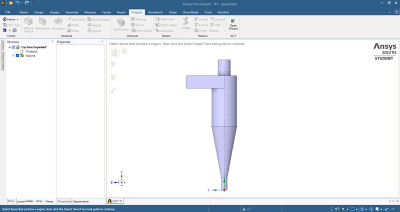
• Extract the fluid domain by using the volume extract option under prepare menu by selecting the inside edges of the model.

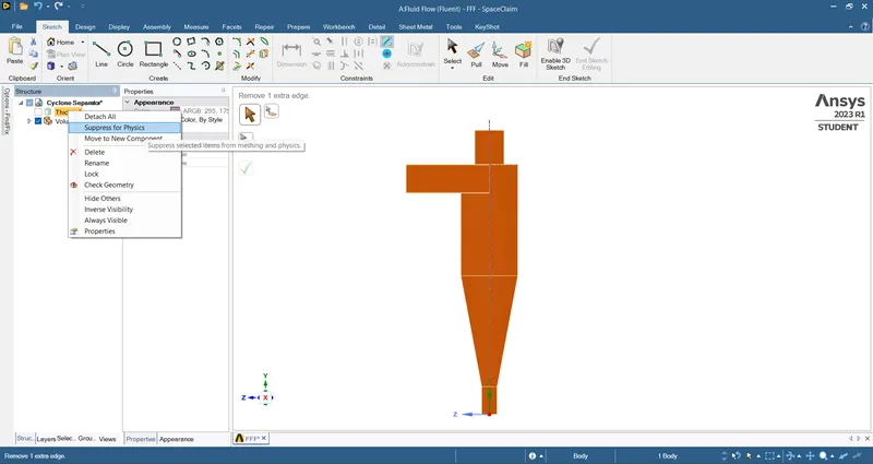
• Suppress the solid part by using suppress for physics option as it is not required for simulation.

Mesh:

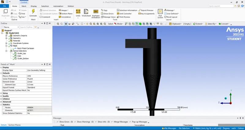
• Select Cartesian method under Mesh>Method option and select the whole body and mesh it with an element size of 0.5 mm.

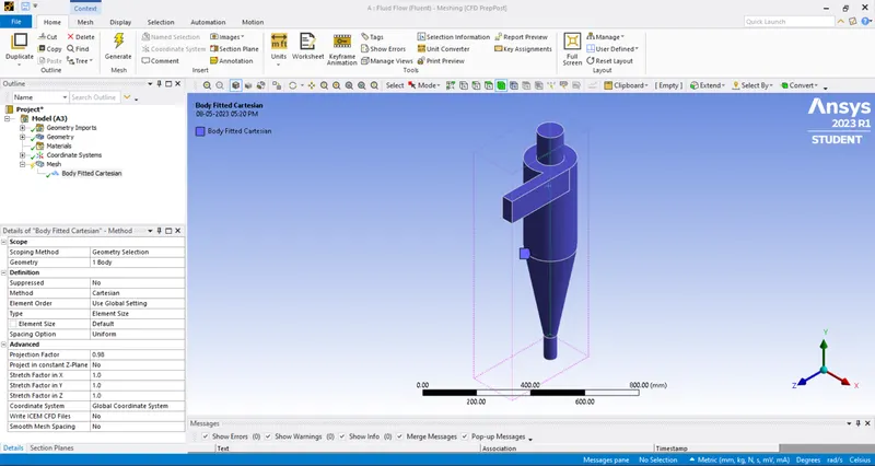
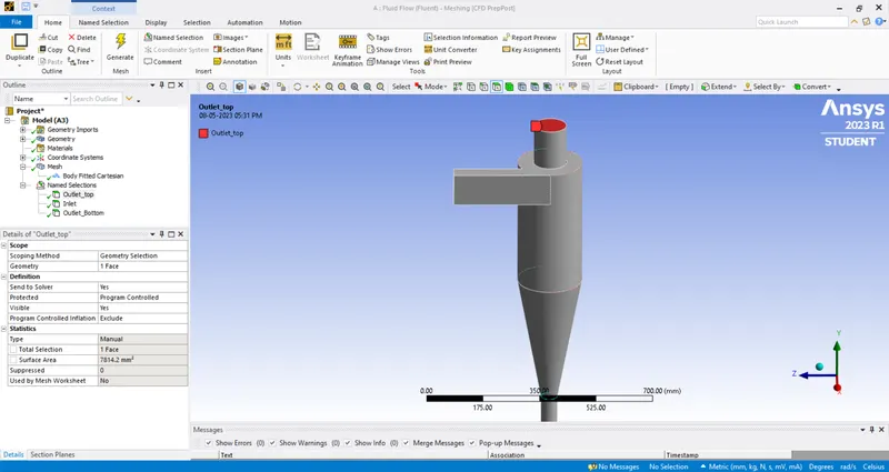
• Create named selections by using the 'N" button and naming the parts appropriately.

Setup:

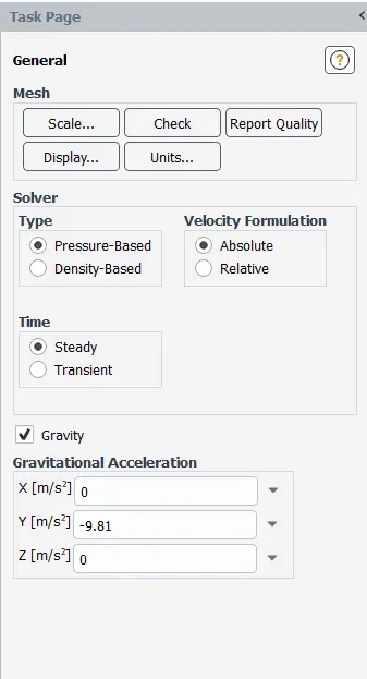
• Under general settings, select pressure-Based type solver, Steady time, Gravity and assign Gravitational acceleration as -9.81 m/s² in the Y-axis.

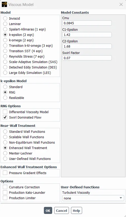
• Under Viscous Model, select RNG k-epsilon model, swirl dominated flow, Enhanced Wall Treatment and click ok.

• Under Discrete Phase Model, increase the Max. Number of steps and create injections.

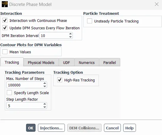
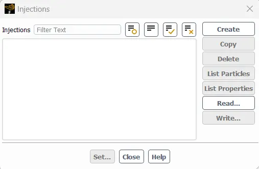
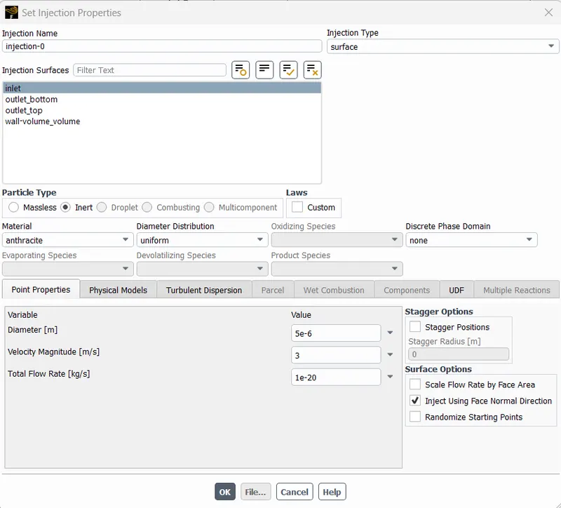
• Select surface injection type and surface as inlet, enable inject using face normal direction and assign the properties appropriately such as particle diameter and velocity magnitude.

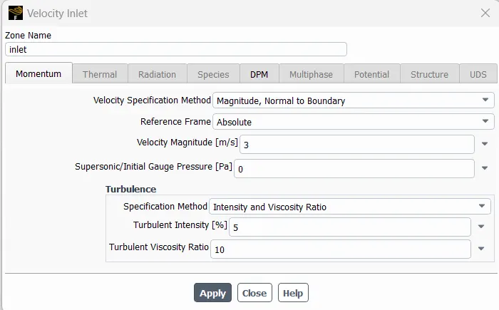
• Assign the Boundary Conditions appropriately, select different Discrete Phase Modules and required for the simulation.

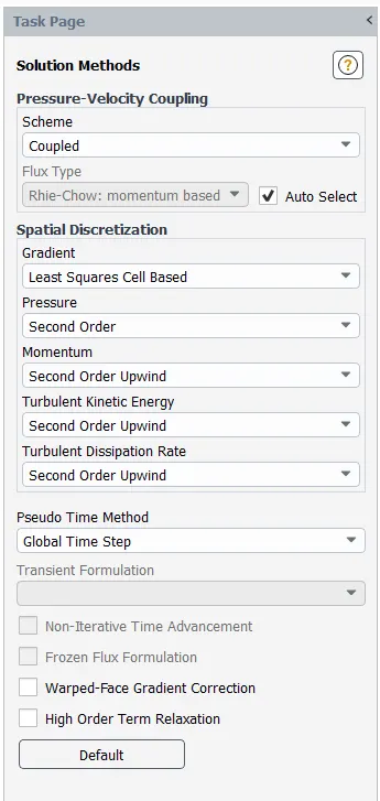
• Select Coupled scheme method, Second order pressure, Second order upwind for Momentum, Turbulent Kinetic Energy and Turbulent Dissipation Rate, Global time Step for Pseudo Time Method under Solution Methods tab.

• Under Solution Initialization, select Standard Initialization computing from all-zones and click Initialize.

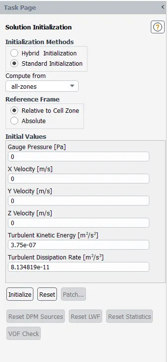
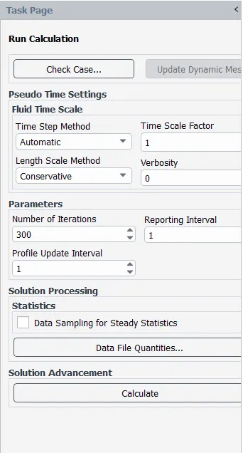
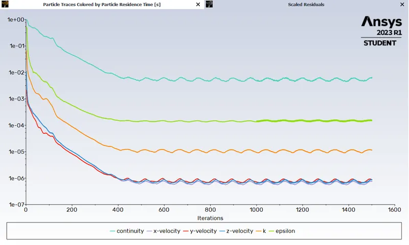
• Run calculation using appropriate number of iterations until the solution is converged.

RESULTS:

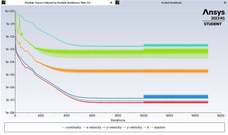
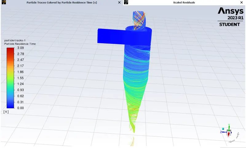
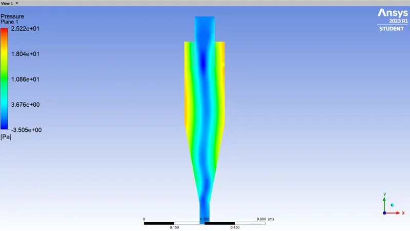
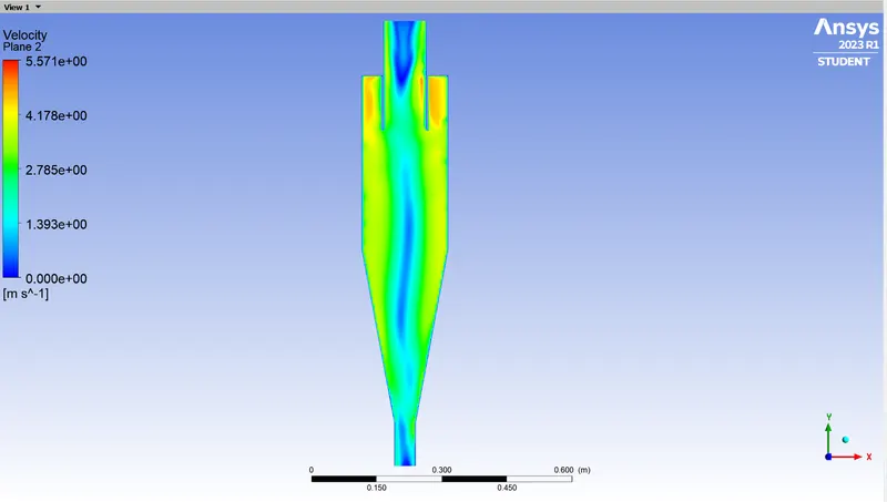
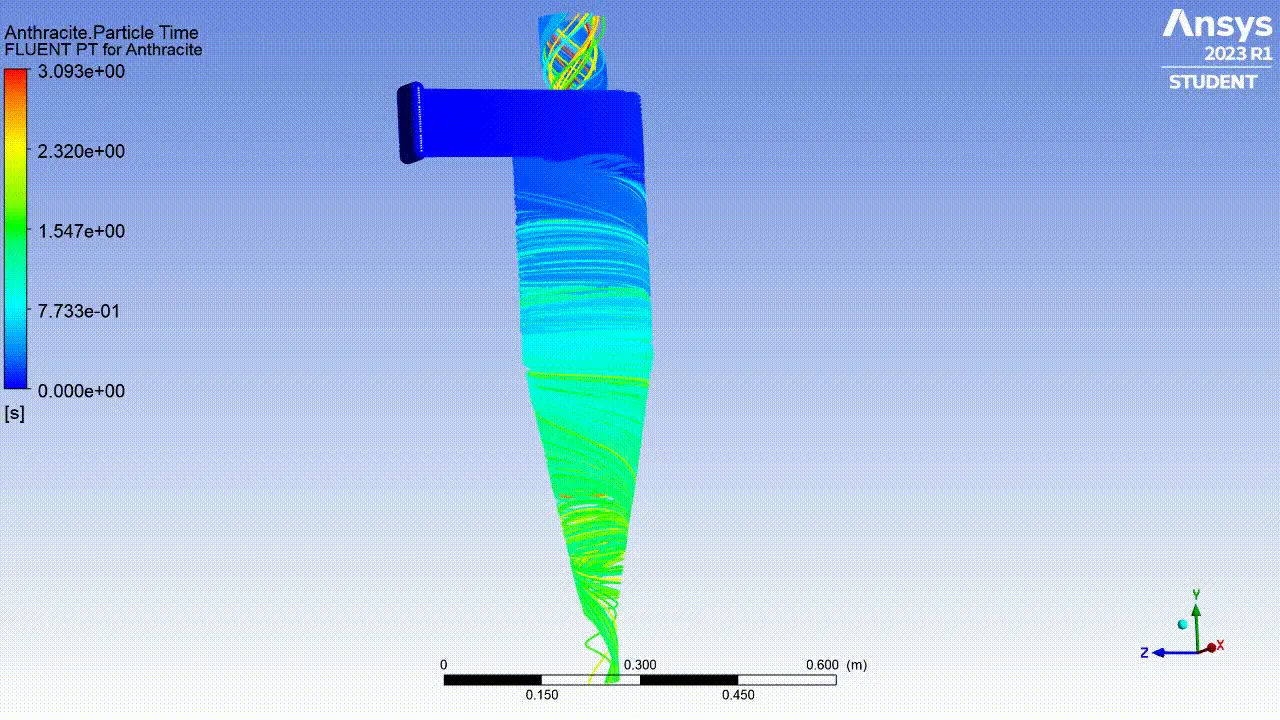
Case 1: Particle diameter as 5 μm and flow velocity as 3 m/sec.

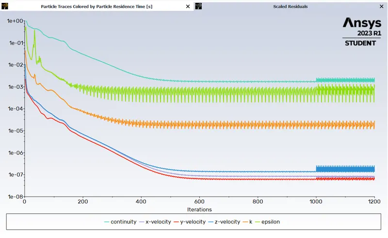
Scaled Residuals:

Particle Residence Time:

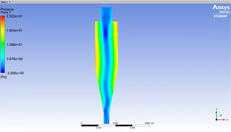
Pressure Contour:

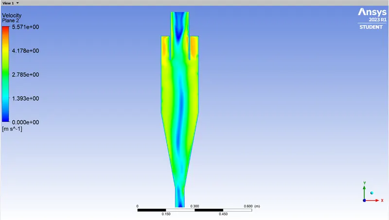
Velocity Contour:

Particle data:

Animation:

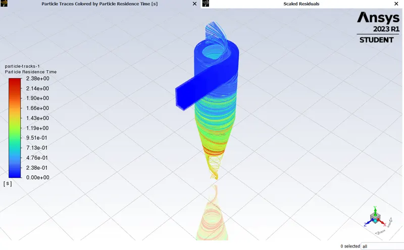
Case 2: Particle diameter as 3 μm and flow velocity as 3 m/sec.

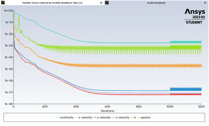
Scaled Residuals:

Particle Residence Time:

Pressure Contour:

 

Velocity Contour:

Particle data:

Animation:

Case 3: Particle diameter as 1 μm and flow velocity as 3 m/sec.

Scaled Residuals:

Particle Residence Time:

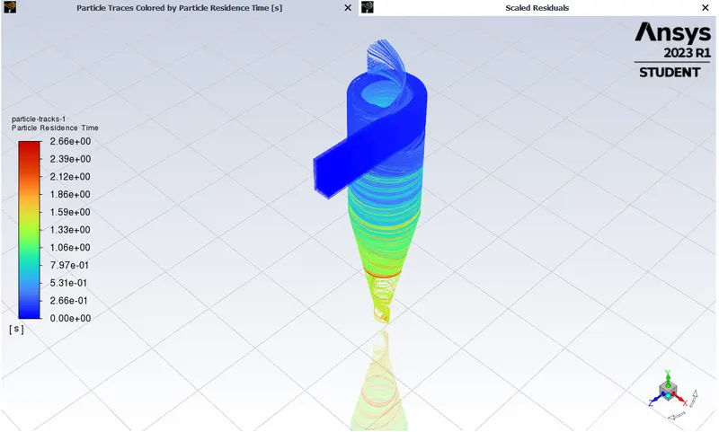
Pressure Contour:

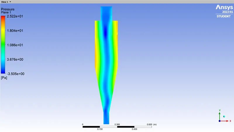
Velocity Contour:

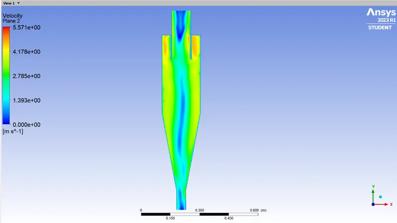
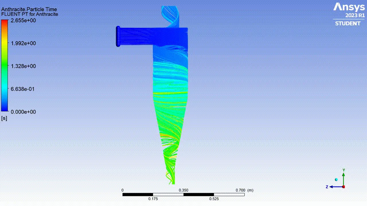
Particle data:

Animation:

Case 4: Particle diameter as 5 μm and flow velocity as 5 m/sec.

Scaled Residuals:

Particle Residence Time:

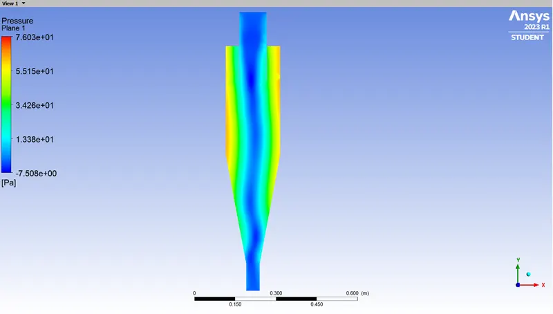
Pressure Contour:

Velocity Contour:

Particle data:

Animation:

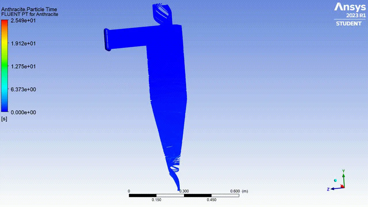
Case 5: Particle diameter as 5 μm and flow velocity as 1 m/sec.

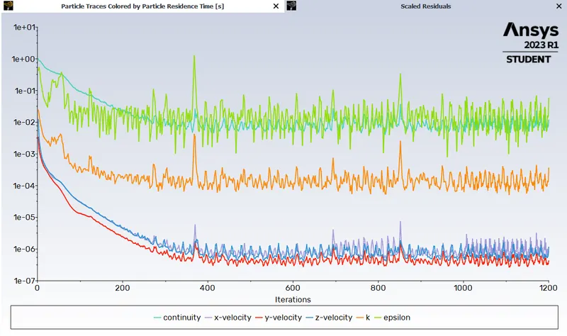
Scaled Residuals:

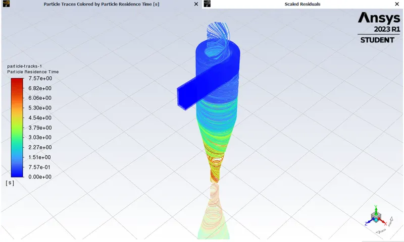
Particle Residence Time:

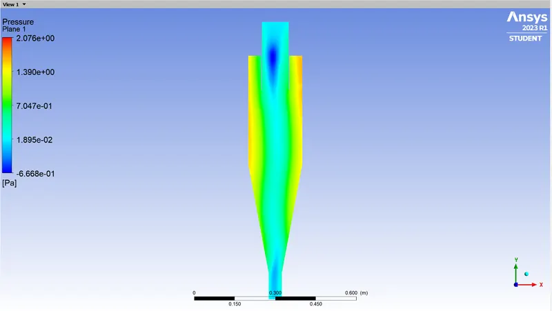
Pressure Contour:

Velocity Contour:

Particle data:

Animation:

CONCLUSIONS:

• The Separation Efficiency and Pressure Drop of all the cases are calculated and shown in the following table:

Cases	Particle Diameter (μm)	Flow Velocity (m/sec)	Separation Efficiency (η)	Pressure Drop (Pa)
1	5	3	71.43%	26.14
2	3	3	82.27%	26.14
3	1	3	81.75%	26.14
4	5	5	72.22%	76.49
5	5	1	80.69%	2.32

• The case with particle diameter as 3 μm and flow velocity of 3 m/sec has the highest separation efficiency.
• The case with particle diameter as 5 μm and flow velocity of 5 m/sec has the highest pressure drop.
• The case with particle diameter as 5 μm and flow velocity of 1 m/sec has the lowest pressure drop of 2.32 Pa.
• The pressure drop in the cases with flow velocity of 3 m/sec is nearly same.
• As the flow velocity decreases the pressure drop also decreases.
• All the solutions for the simulation has achieved convergence.