Week 4 - CHT Analysis on Exhaust port

AIM: Perform the heat transfer analysis using ANSYS-Fluent software for the given exhaust port problem and use air as the working fluid with velocity of 5 m/s. Consider Inlet and outlet temperature as 700 K and 300 K respectively. Take the wall heat transfer coefficient as 20 W/m²K.

Expected results:

• Give a brief description of why and where a CHT analysis is used.
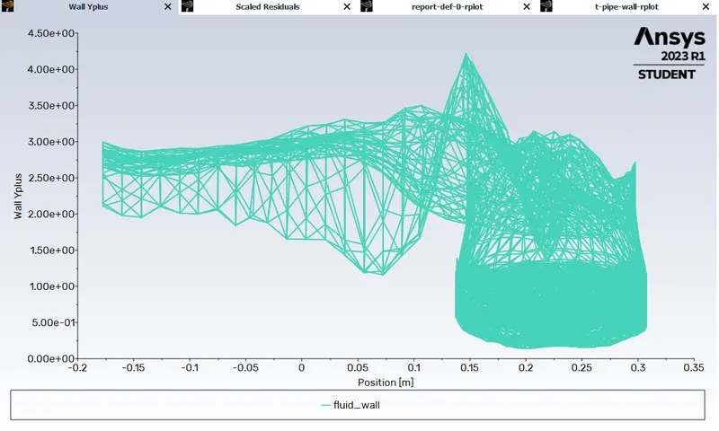
• Maintain the y+ value according to the turbulence model and justify the results.
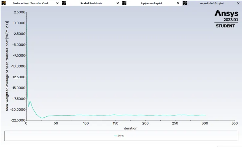
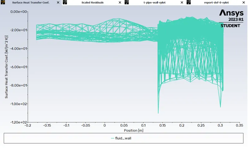
• Calculate the wall/surface heat transfer coefficient on the internal solid surface & show the velocity & temperature contours in appropriate areas.
• How would you verify if the HTC predictions from the simulations are right? On what factors does the accuracy of the prediction depend on?

INTRODUCTION:

The Conjugate Heat Transfer (CHT) analysis type allows for the simulation of heat transfer between solid and fluid domains by exchanging thermal energy at the interfaces between them. It involves solving the heat transfer equations for both the fluid and the solid regions simultaneously, taking into account the heat transfer between them. The fluid flow is solved using the Navier-Stokes equations, and the heat transfer equations are solved using the energy equation. The solid region is modeled as a three-dimensional solid, and its thermal behavior is determined by solving the heat conduction equation.

CHT analysis is used in a wide range of engineering applications, such as in the design of heat exchangers, electronic cooling systems, and turbine blades. CHT analysis is an important tool for designing and optimizing systems that involve heat transfer between a fluid and a solid, and it can help ensure that these systems operate efficiently and reliably.

Conjugate Heat Transfer analysis is majorly used in the following applications

1. Aerospace engineering: In the design of aircraft engines, CHT analysis is done to study the heat transfer between the hot gases and the turbine blades. 

2. Automotive engineering: In the design of combustion engines and exhaust systems, CHT analysis is done to study the heat transfer between the combustion gases and the engine components. 

3. Electronics industry: In the design of electronic devices, CHT analysis is done to study the heat transfer between the electronic components and the surrounding fluid.

SOLVING & MODELLING APPROACH:

In this simulation, working fluid i.e. air, is transfered in an exhaust port from inlet at a velocity of 5 m/s to the outlet where the inlet temperature is considered as 700 K and oulet temperature is considered as 300 K and heat transfer coefficient is taken as 20 W/m²K.

PRE-PROCESSING AND SOLVER SETTING:

Geometry:

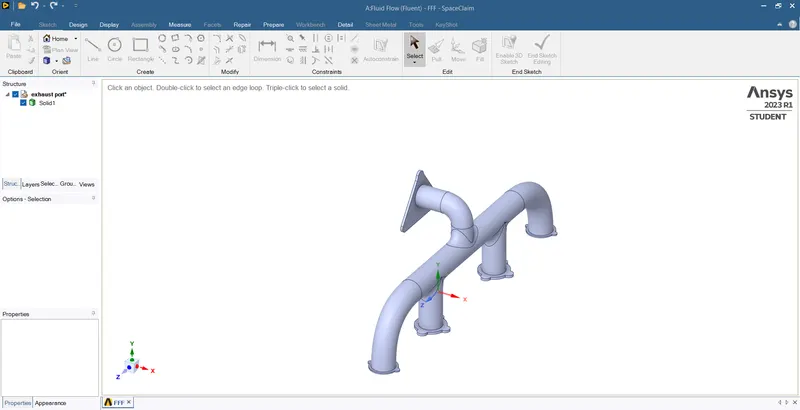
• Run ANSYS 2023 R1 student version and drag Fluid Flow (Fluent) in the project Schematic and then run ANSYS Space Claim by selecting it from Geometry. Then import the Exhaust port by using the option File> Open>exhaust port.SLDPRT.

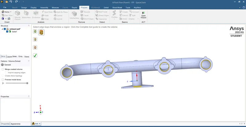
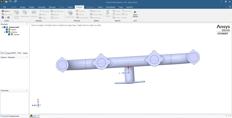
• Select Prepare>Volume extract to separate the internal pipe section which is a fluid domain with the external pipe section which is a solid domain.

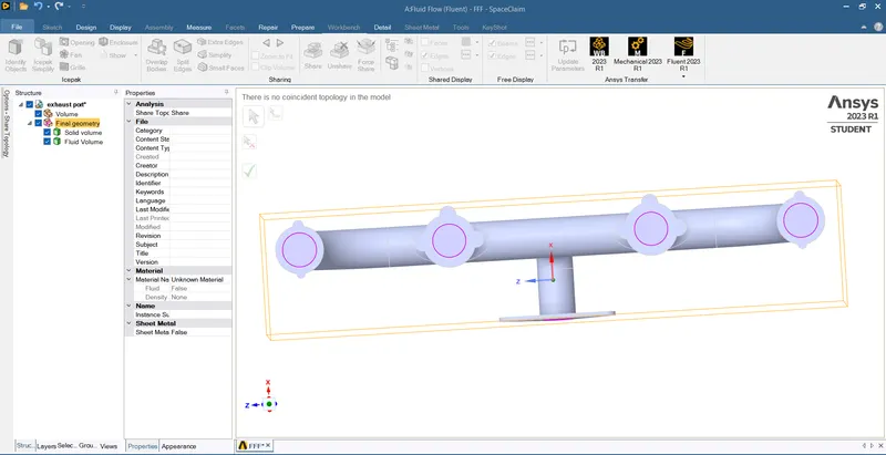
• Share topology between the internal pipe section and external pipe section so that the meshing is properly shared between them.

Mesh:

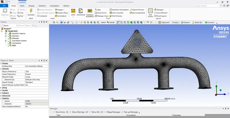
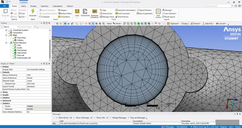
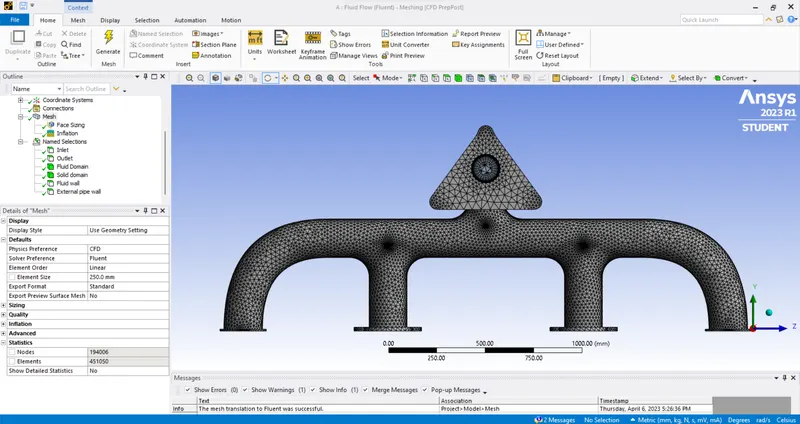
• Generate a coarse mesh after loading the exhaust port in the meshing window with an element size of 250 mm. Then name the different sections of the geometric body such as inlet, outlet, fluid domain, solid domain, fluid wall and external pipe wall by selecting the appropriate body/sides by using the named selection option or by clicking 'N" after selecting the side.

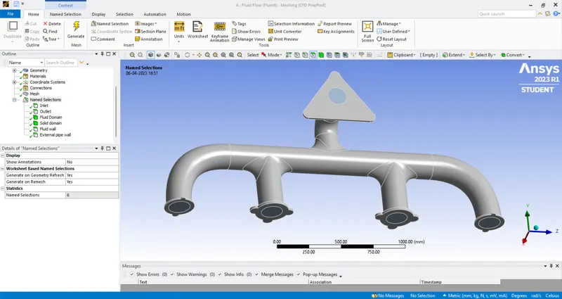
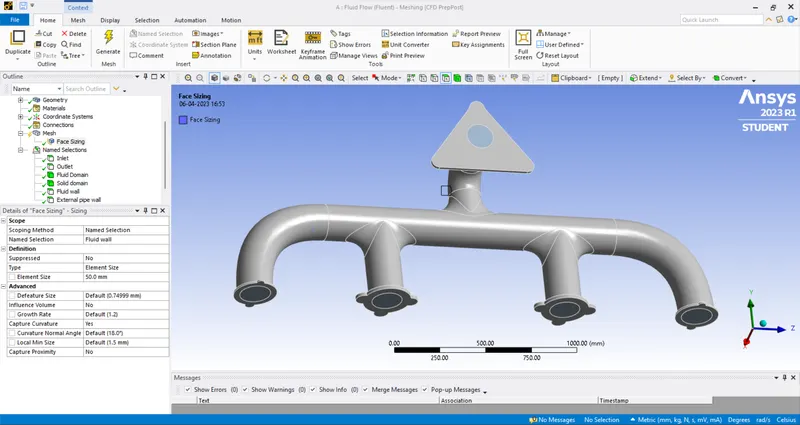
• Create Face sizing mesh for the fluid wall by selecting named selctions. Select Mesh>Insert>Sizing , then select appropriate body and element size as necessary and then generate mesh.                                 

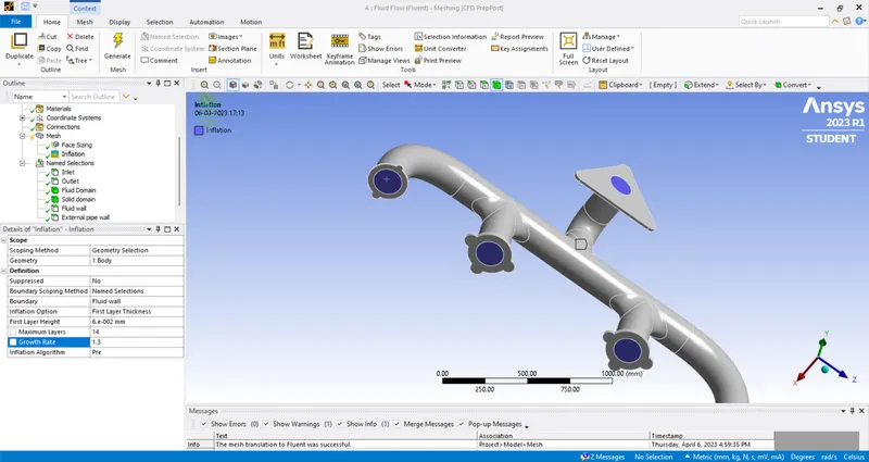
• To create an Inflation layer, calculate the first layer thickness by using Y+ Calculator by providing the appropriate values. The desired Y+ is taken as 1 and growth rate is taken as 1.3, first layer height is taken as 0.00006. It is taken by comparing Prism Layer Total Thickness and Boundary Layer Thickness, where Prism Layer Total Thickness must be greater tan the Boundary Layer Thickness.

SETUP:

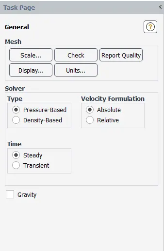
• Under general settings, selected pressure-Based type solver and steady time.

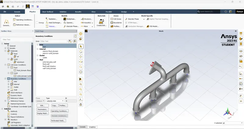
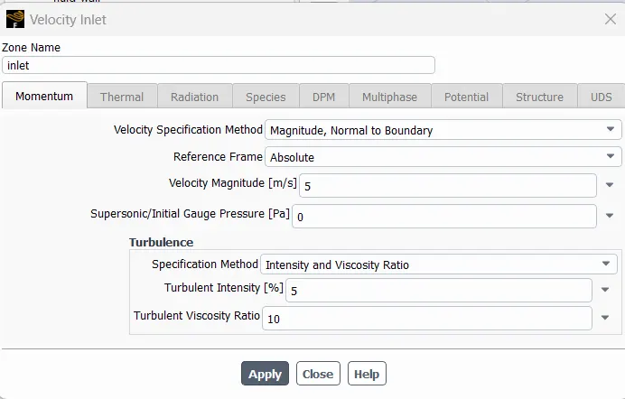
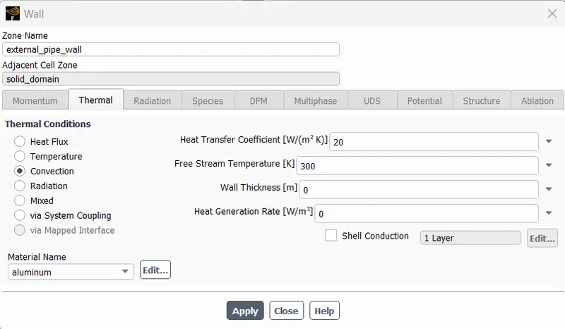
• Select Materials as air under fluid and aluminum under solid and set boundary conditions, where the inlet velocity will be 5 m/s, inlet temperature will be 700 K, the heat transfer coefficient will be 20 W/m²K and oulet temperature will be 300 K.

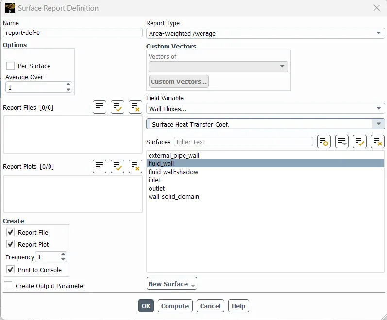
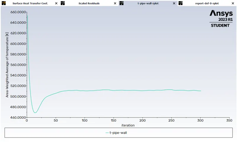
• Under solution tab, select Definitions> New>Surface Report>Area-Weighted Average and select Wall Fluxes and surface heat transfer coefficient for fluid wall, Definitions> New>Surface Report>Area-Weighted Average and select Temperature for external pipe wall.

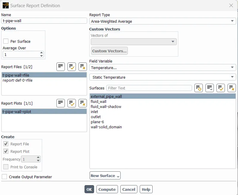
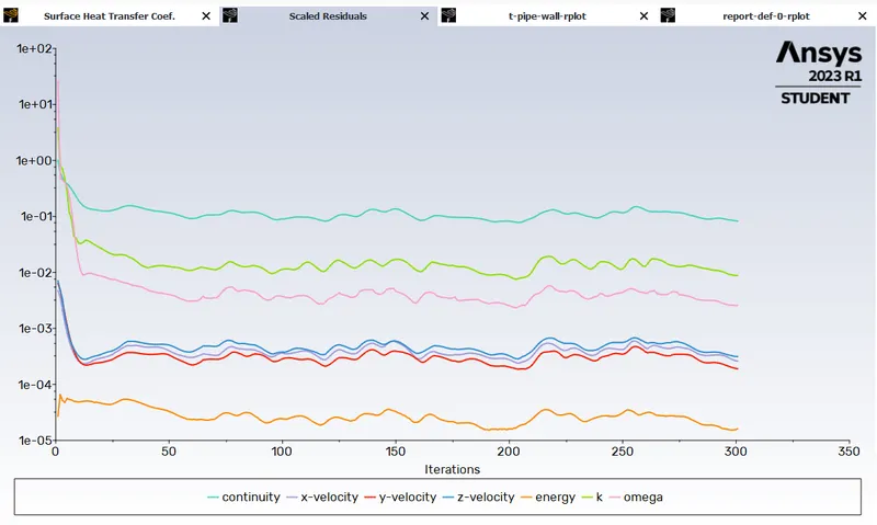
• For Initialization select Hybrid Initialization and then click initialize and then run necessary number of iterations until the solution is converged.

RESULTS:

Scaled Residuals:

Heat Transfer Coefficient plot:

 

Temperature Plot:

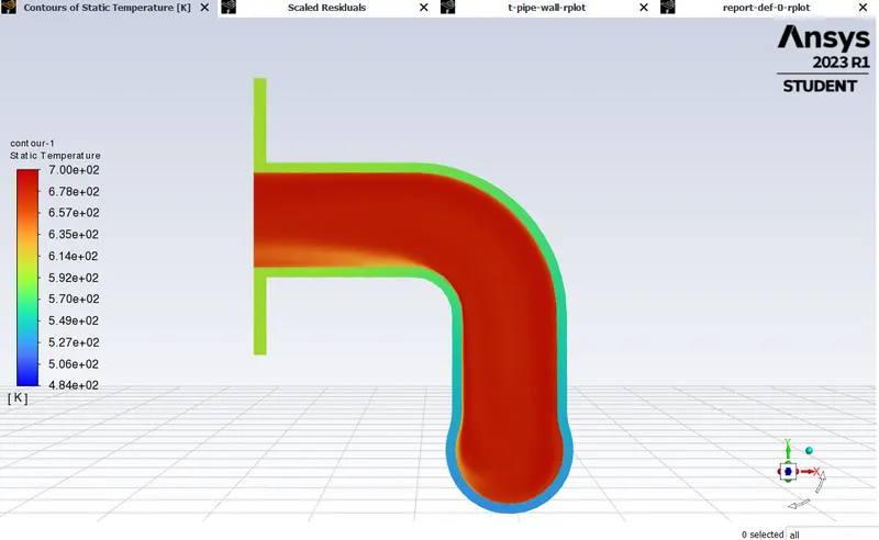
Temperature Contour:

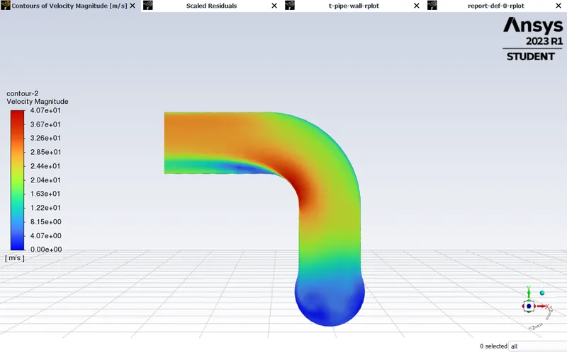
Velocity Contour:

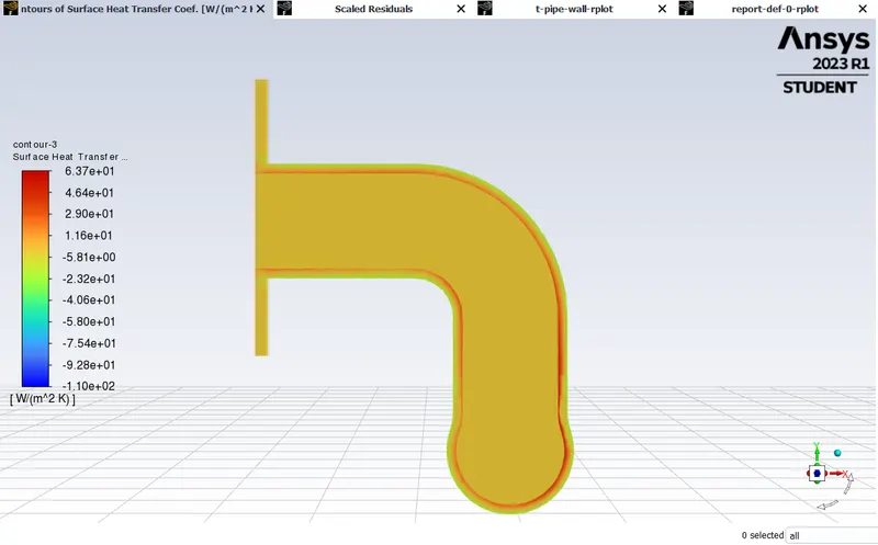
Surface Heat Transfer coefficient:

Wall Y Plus:

Surface Heat Transfer Coefficient:

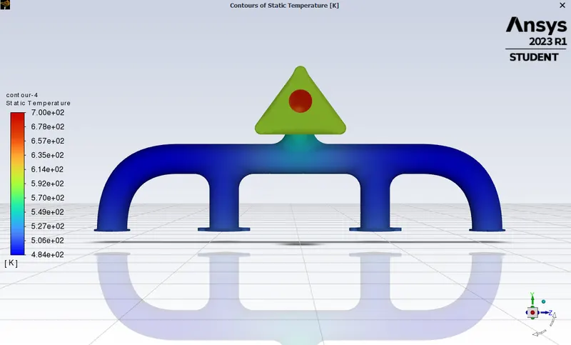
Overall temperature contour:

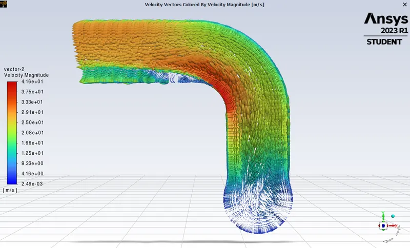
Velocity Vector:

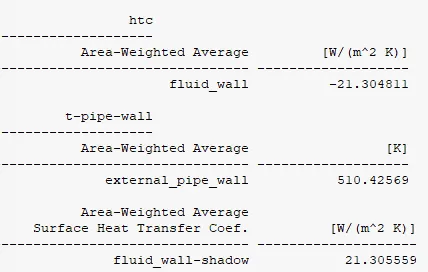
Heat Transfer Coefficient:

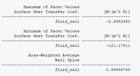
Y Plus nearly equal to 1:

Verifying the HTC predictions from the simulations:

• The Nusselt number is the ratio of convective heat transfer to conductive heat transfer within a fluid region.

                    

where h is the  convective heat transfer coefficient of the flow, L is the characteristic length, k is the thermal conductivity of the fluid.

• Nusselt number is related to Reynolds number by this mathematical equation:

                                                 

Where ,

                           

              and u is the flow speed (m/s)

• We observed heat transfer coefficinet is directly proportional to the Reynolds number as well as the velocity. So with increase in velocity the convective heat transfer coefficient will also increase. Therefore, increase in the Reynold's number will lead to increment of overall convective heat transfer coefficient.

CONCLUSIONS:

The factors in which the accuracy of the prediction depends are:

• The topology should be shared, as because the meshing will be properly connected with each other through the nodes. With proper meshing there will be better calculations.
• Inflation layers should be created with the help of Y plus calculator so as to achieve proper flow capturing in the fluid wall as the meshing near the wall will be properly refined.
• Setting appropriate boundary conditions.
• Selecting K omega SST model for the simulation as it gives better results near the wall.