Week 8 - Simulating Cyclone separator with Discrete Phase Modelling

Aim: To perform simulation on cyclonic separator and to calculate the presure drop and the separation efficiency for five different cases by varying particle diameter and velocity.

Introduction: Cyclonic separators are separation devices which separate the particulate matter from the flue gases. In same scale industries it may also be refereed as dust separators. It uses the principle of inertia to separate particles from the flue gases. It is used in many applications due to the low cost, simple design and high efficiency. Generally two types are there: gas cyclone separators and hydrocyclone separators. Gas cyclone separators are used to separate the particles from the gas which hydrocyclone separators are used to separate fluids of different densities. Gas separators are again of two types: axial and reverse flow gas separators. Reverse flow gas separators are most widely used in industries and in this project we consider it.

Theory: Cyclonic separators consists of one inlet and two outlets. Through inlet we sent the air mixed with particle of low diameter. The flow is tangential and the swirling action takes place. The principle of inertia takes place. Inertia is nothing but the ability of a body to stay in its orginal state unless acted by external force. The high inertia particle will move down through outlet trap, while low inertia particle will move up through outlet escape. The two important parameters are separation efficiency and pressure drop. It is found the efficiency is also function of particle size ; with larger particle size will have higher efficiency compared to lower particle size. The pressure drop is also important as high pressure drop can leads to higher operational costs.

Generally in multiphase flow we follow two approaches: Euler- Langrange approach and Euler - Euler approach. In this project we will use discrete phase model which follows the Euler Langrange approach. Here fluid phase is treated as continuum by solving Navier stokes equation; while dispersed phase is solved by tracking large number of bubbles, particles or droplets through calculated flow field. In DPM we will follow one assumption: the dispersed second phase occupies very low volume fraction. This model is ideal for spray dryers, particle laden flow etc. We will calculate the pressure drop and separation efficiency in this project. Cyclonic separators are used in industrial applications like power generation, gas turbine, chemical processes and so on. The highly swirling flow inside cyclone is complex including interaction between fluid phases and the particulates.

The empirical models used to calculate cyclone separator efficiencies are

Iozia and Leith Model:

This model is base on the force balance and it assumes that a particle carried by the vortex endures influence of two forces: centrifugal force and flow resistance.

Li and Wang Model :

The Li and Wang model includes particle bounce or reentrainment and turbulent diffusion at the cyclone wall. A two dimensional analytical expression of particle distribution in the cyclone is obtained. Li and Wang model was developed based on the following assumptions:

• The radial particle velocity and the radial concentration profile are not constant for uncollected particles within the cyclone.

Koch and Licht Model:

Koch and Licht collection theory recognized the inherently turbulent nature of cyclones and the distribution of gas residence times within the cyclone. Koch and Licht described particle motion in the entry and collection regions with the additional following assumptions:

• The tangential velocity of a particle is equal to the tangential velocity of the gas flow, i.e. there is no slip in the tangential direction between the particle and the gas.
• The tangential velocity is related to the radius of cyclone by: uRⁿ = constant.

Lapple Model:

Lapple model was developed based on force balance without considering the flow resistance. Lapple assumed that a particle entering the cyclone is evenly distributed across the inlet opening. The particle that travels from inlet half width to the wall in the cyclone is collected with 50% efficiency.

Solving and modelling approach:

First the model is imported into the spaceclaim of Fluent of Ansys Workbench. Then we have to add fluid domain inside using volume extract option. Then we will suppress the solid for physics. Then we will perform meshing. First we will go with the default mesh, then we will change the base element size to 5 mm,and do the meshing. Then we will do the automatic method with body fitted cartesian. Since the geometry is of basic cone and cylinder shape we have gone with the structured mesh. Then we will do the named selections : inlet reflect, outlet escape and outlet trap. Then we will update the mesh.

Then we will do the processing using fluent solver. Here we will enable the pressure based solver with gravity enabled as -9.81 m/s2 in negative y direction. Then we will select the models: we go with k epsilon RNG standard wall function turbulence model with swirl mode on. Then we will enable the discrete phase on: then we will enable the interaction with continous phase and high resolution tracking. Then we will go with the injections: create it and give the material name as anthracite. Then the velocity is given in x direction: first three cases we will use 3 m/sec, and we will the particle diameter as 1 micrometer in the first case. Then we will save it and we will give the boundary conditions. We will give the velocity inlet as 3 m/sec , and enable as reflect; while we have two pressure outlets: first is pressure outlet with escape mode and second is pressure outlet with trap mode. Now we will select the methods: we use coupled pressure velocity coupling, then we will use second order upwind turbulent kinetic energy and second order upwind turbulent dissiparion rate. Then we will do the standard intialization with compute from inlet and run for 350 iterations.

Preprocessing and solver settings:

(i) Geometry creation

We will import the geometry of stp file format into spaceclaim of the fluent of ansys workbench. Then we will add fluid domain inside using volume extract command. Then we will suppress the solid.

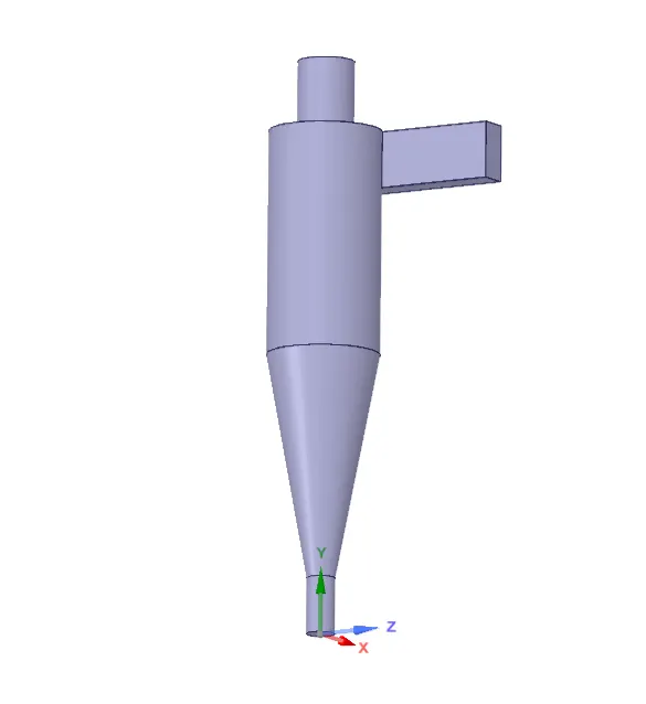
Fig 1 : geometry of model

(ii) Meshing

Now we will do the preprocessing, with base element size of 5 mm, and we will enable automatic body fitted cartesian.

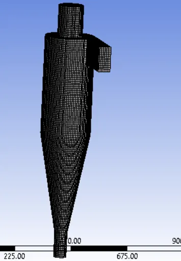
Fig 2 : meshing of model

Then the named selections are given: inlet reflect, outlet escape, outlet trap. Then update the mesh.

(iii) Fluent solver processing

We will enable the pressure based solver with gravity as -9.81 m/s2 in y direction. Then the models are selected

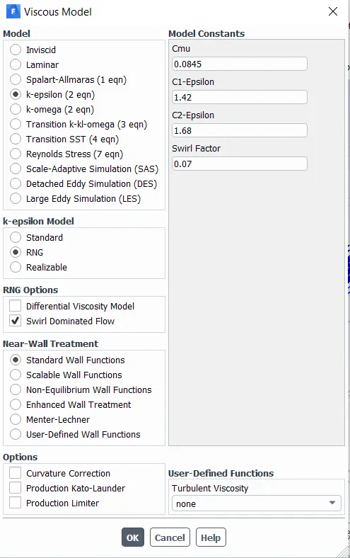
Fig 3 : selecting turbulence model

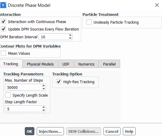
Fig 4 : selecting discrete phase model

We are using k epsilon RNG model with standard wall function. RNG mode is generally selected for swirl induced flow. Then we will select discrete phase model with interaction with continous phase enabled mode. Then the injections are enabled: with particle as anthracite material ; diameter as 1 micrometer and velocity as 3 m/sec.

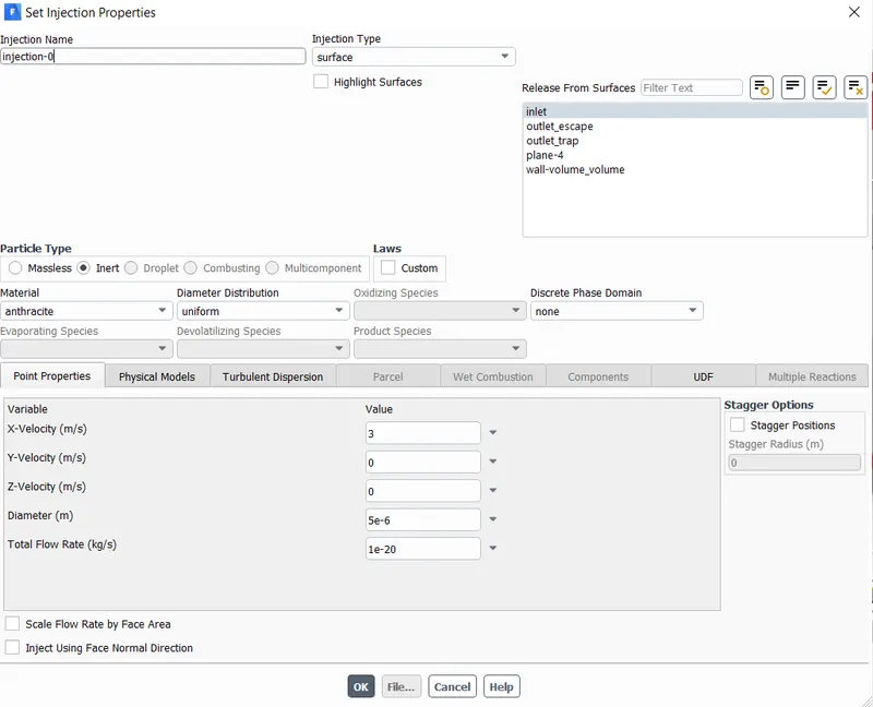
Fig 5 : selecting injection

Now the boundary conditions are given.

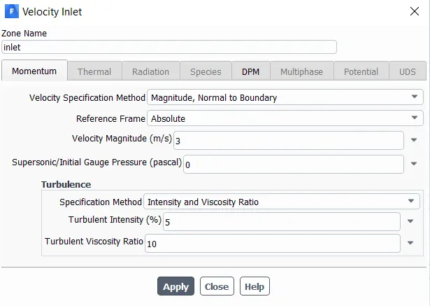
Fig 6 : selecting velocity inlet

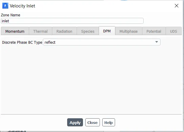
Fig 7 : selecting inlet phase type as reflect

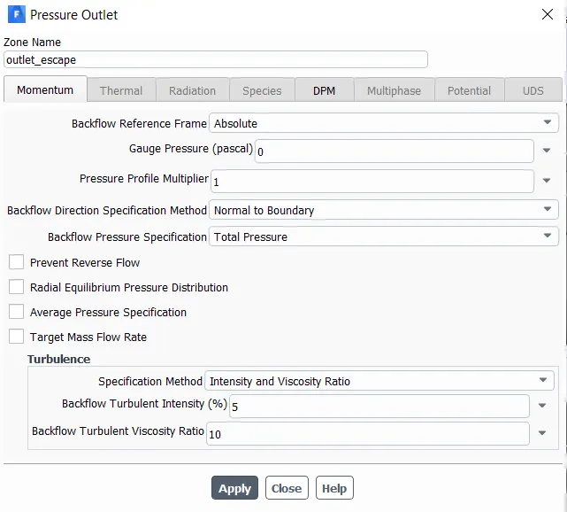
Fig 8 : selecting pressure outlet

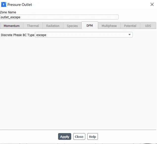
Fig 9 : selecting pressure outlet one discrete phase type as escape

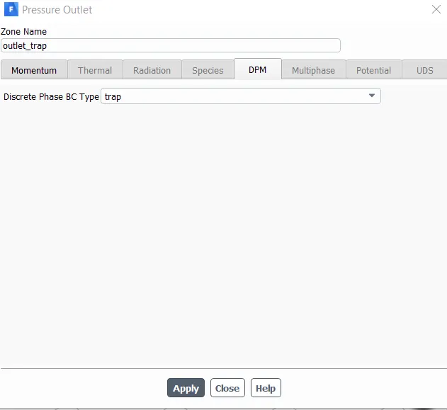
Fig 10 : selecting pressure outlet two discrete phase type as escape

Outlet one is at the top where the light fluid (air ) will escape; hence escape mode is given in DPM phase type; while for outlet two which is at the bottom where we will trap the anthracite particle , hence we will enable outlet as trap DPM phase type.

Now we will do the intialization. For that we will do the standard intialization.

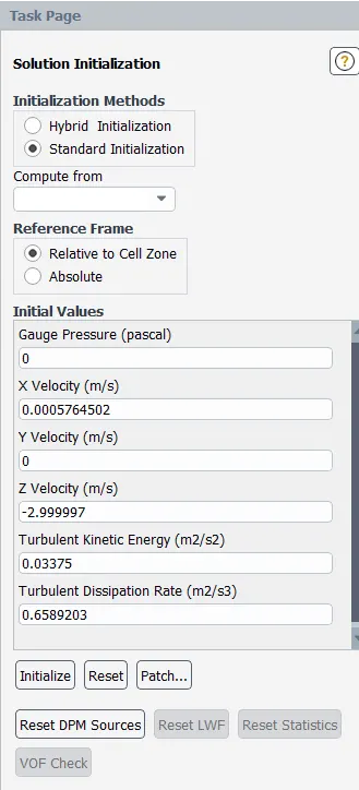
Fig 11 : selecting standard intialization

Results:

(i) Residual contours

(a) For particle diameter of 1 micrometer and velocity of 3 m/sec

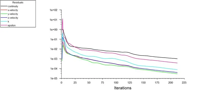
Fig 12 : Residual plot for case 1

(b) For particle diameter of 3 micrometer and velocity of 3 m/sec

Fig 13 : Residual plot for case 2

(c) For particle diameter of 5 micrometer and velocity of 3 m/sec

Fig 14 : Residual plot for case 3

(d) For particle diameter of 5 micrometer and velocity of 1 m/sec

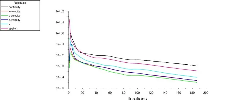
Fig 15 : Residual plot for case 4

(d) For particle diameter of 5 micrometer and velocity of 5 m/sec

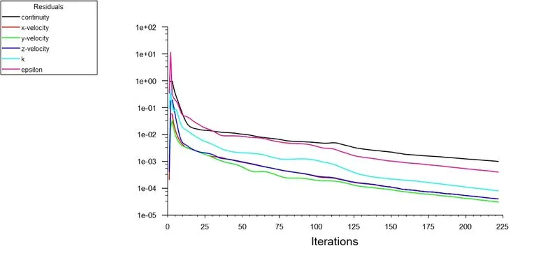
Fig 16 : Residual plot for case 5

(ii) Velocity contour

(a) For particle diameter of 1 micrometer and velocity of 3 m/sec

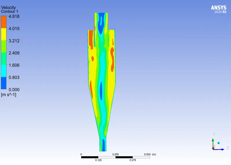
Fig 17: velocity contour for case 1

(b) For particle diameter of 3 micrometer and velocity of 3 m/sec

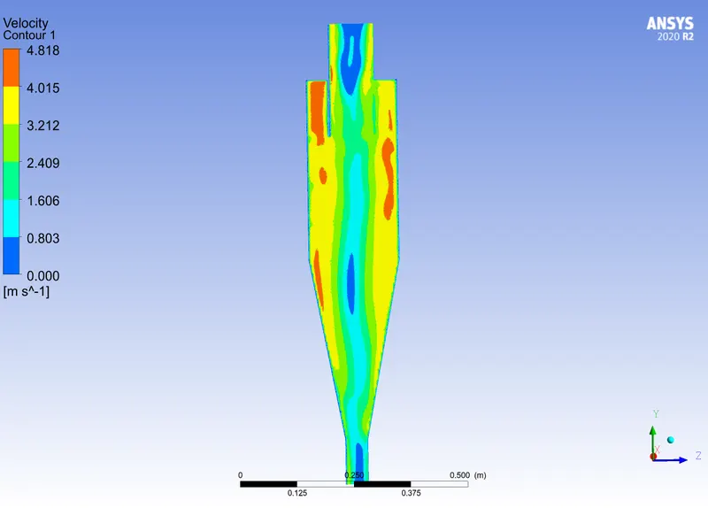
Fig 17: velocity contour for case 1

(c) For particle diameter of 5 micrometer and velocity of 3 m/sec

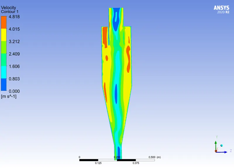
Fig 19: velocity contour for case 3

(d) For particle diameter of 5 micrometer and velocity of 1 m/sec

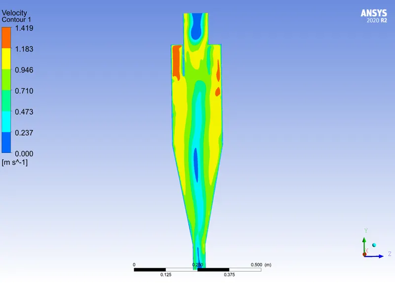
Fig 20: velocity contour for case 4

(e) For particle diameter of 5 micrometer and velocity of 5 m/sec

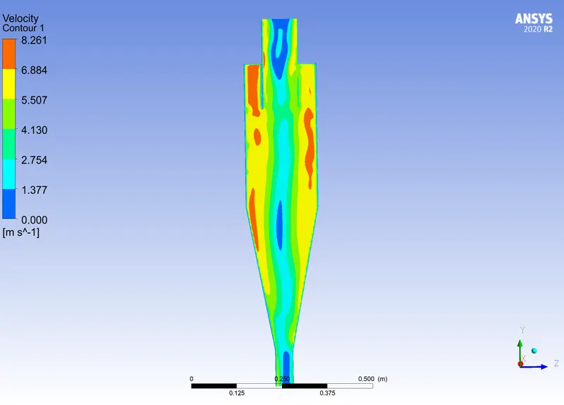
Fig 20: velocity contour for case 5

(iii) Pressure contour

(a) For particle diameter of 1 micrometer and velocity of 3 m/sec

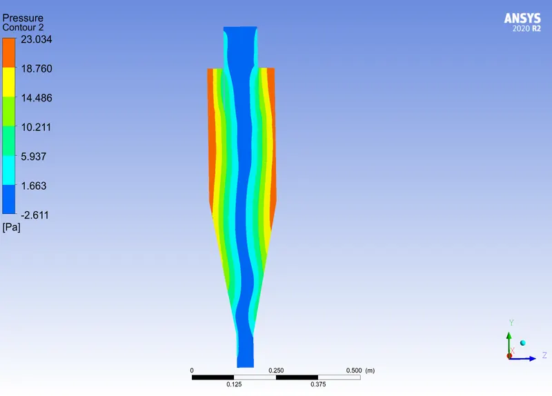
Fig 21 pressure contour for case 1

(b) For particle diameter of 1 micrometer and velocity of 3 m/sec

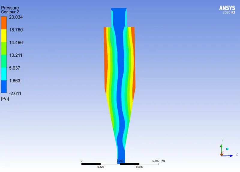
Fig 22 pressure contour for case 2

(c) For particle diameter of 5 micrometer and velocity of 3 m/sec

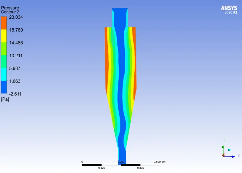
Fig 23 pressure contour for case 3

(d) For particle diameter of 5 micrometer and velocity of 1 m/sec

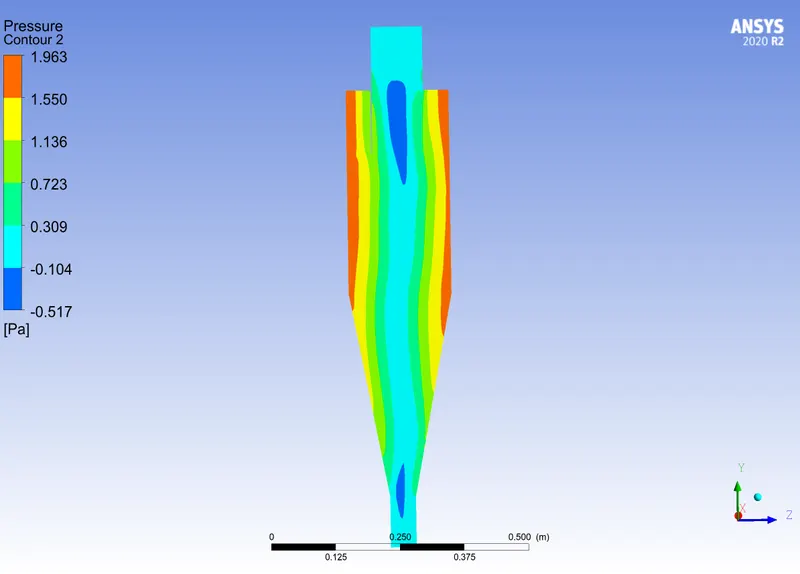
Fig 24 pressure contour for case 4

(e) For particle diameter of 5 micrometer and velocity of 5 m/sec

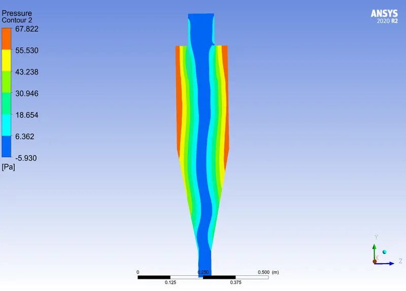
Fig 25 pressure contour for case 5

(iii) velocity vector

(a) For particle diameter of 1 micrometer and velocity of 3 m/sec

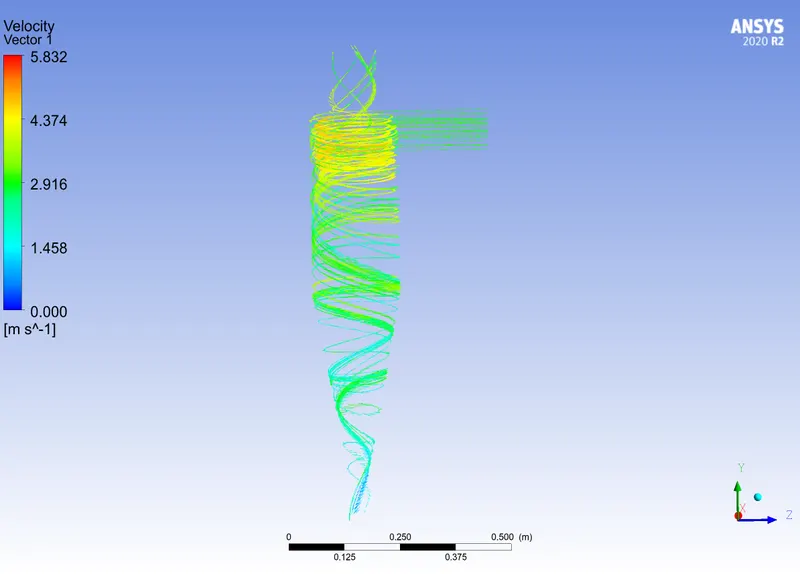
Fig 26 velocity vector contour for case 1

(b) For particle diameter of 3 micrometer and velocity of 3 m/sec

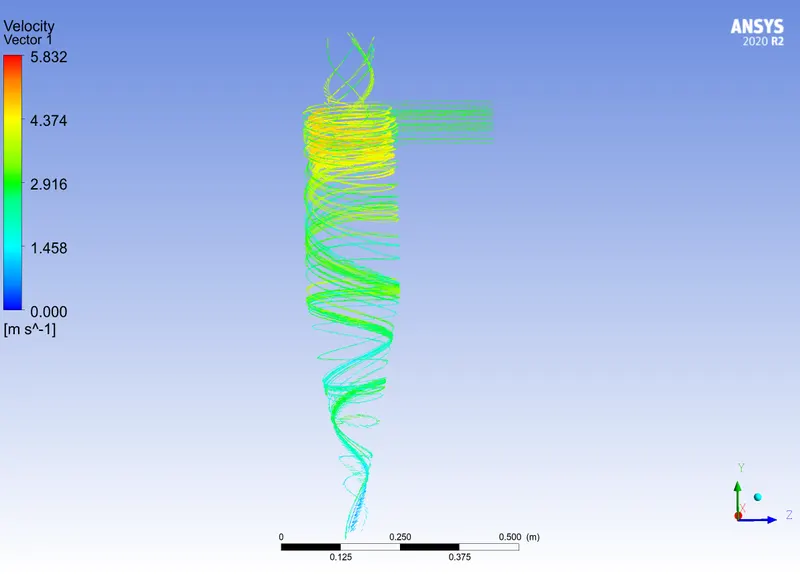
Fig 27 velocity vector contour for case 2

(c) For particle diameter of 5 micrometer and velocity of 3 m/sec

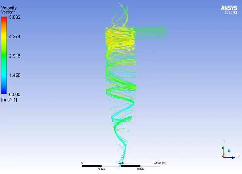
Fig 28 velocity vector contour for case 3

(d) For particle diameter of 5 micrometer and velocity of 1 m/sec

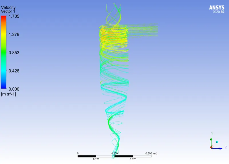
Fig 29 velocity vector contour for case 4

(d) For particle diameter of 5 micrometer and velocity of 5 m/sec

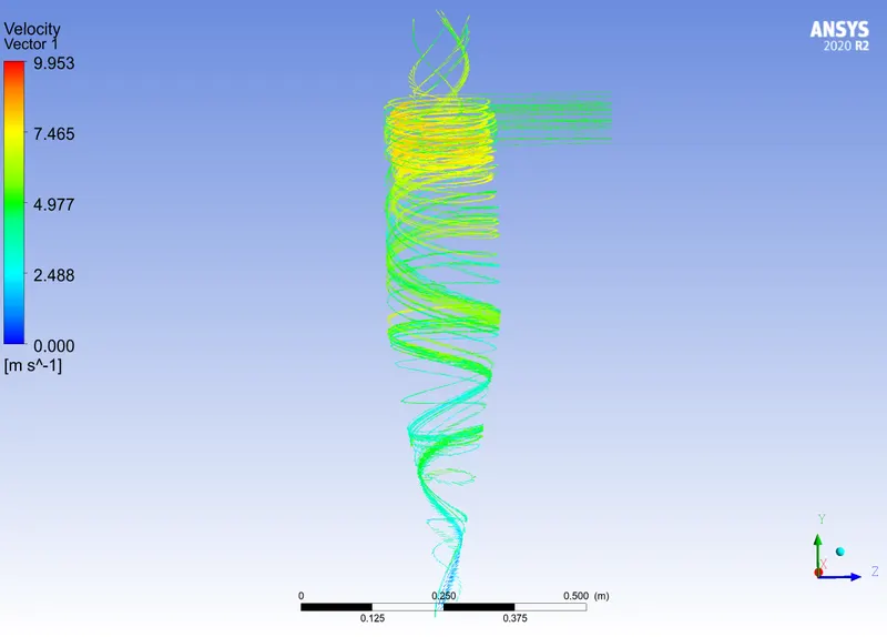
Fig 30 velocity vector contour for case 5

Conclusions:

We have performed simulations for five different cases by varying the particle diameter and velocity and its effect on the pressure drop and separation efficiency is calculated.

S.No	Partcle diameter (micrometer)	Velocity (m/sec)	Pressure drop (Pa)	Particles tracked	Particles trapped	Separation efficiency (%)
1	1	3	26.87	378	163	43.12
2	3	3	26.87	378	127	33.5
3	5	3	26.87	378	200	52.91
4	5	1	2.45	378	252	66.6
5	5	5	77.5	378	29	7.67

• From the above it is clearly observed that the pressure drop is increasing with increasing the velocity; which can increase the operating cost.
• The separation efficiency is the lowest i.e 7.67% for the highest velocity. and the separation velocity is highest i.e 66.6 % for the lowest velocity of 1 m/sec.
• The particle diameter is also have an effect on the separation efficiency and the pressure drop.