Week 2 - Flow over a Cylinder.

Aim: To simulate the flow of air over the cylinder for various reynolds number of 10, 100, 1000, 10000 and 100000 in the steady case and obtain the coefficient of lift, coefficient of drag, and vertex average velocity in all the cases; similarly run the unsteady case with reynolds number of 100 and obtain the strouhal number.

Introduction: The flow of air over the cylinder comes under the external flow problem. If we give more emphasis for pressure drop and flow rate in the internal flow problems, then in external flow problems we give more importance to the lift and drag forces. If the force is exerted by the fluid on the solid in the direction of fluid flow it is called as drag force, and if the force is in the direction perpendicular to the fluid flow it is called as lift force. Generally drag is unnecessary and we have to minimise it. The drag and lift forces arises because of the pressure stresses and wall shear stresses. Pressure stresses is in direction normal to the surface , while wall shear stresses is in tangential direction to the surface. Generally we can consider bodies as bluff bodies and streamlined bodies. Flow over cylinder can be considered as flow over bluff bodies. We are observing the karman vortex street phenomena when the Reynolds number exceed a certain value of around 90.

Theory: The drag force can be of two types : pressure drag and friction drag. Pressure drag is because of the pressure difference distribution occuring across the bodies. Pressure drag is more significant in flow over bluff bodies like flow over cylinder. The flow separation phenomena generally occurs in flow over bluff bodies. The flow separation phenomena can also leads to vortex shedding which leads to unnecessary vibrations and stability issues. If we can delay the flow separation, we can reduce the presure drag. By introducing turbulence or mixing, we can delay the flow separation, hence the pressure drag. But if we consider streamline bodies, flow separation occurs lately or may not occur also. The angle of attack is also important here. Here the pressure drag is less and most drag arises from the friction drag. This drag is because of fluid friction, and greater the fluid viscosity greater the friction drag.

Karman vortex street is the repeating pattern of swirling vortices, cause by the process known as vortex shedding, which is responsible for unsteady separation of flow of fluid around bluff bodies. It is responsible for the singing of suspended powerlines and vibration of car antennas at certain speeds. It occurs only at the certain flow velocities typically about Reynolds number greater than 90. Strouhal number is a dimensionless number describing oscillating flow mechanisms.

Strouhal No Sr = fL/u; where f = frequency of vortex shedding, L = characteristic length and u = flow velocity.

The strouhal number variation with reynolds number is considered, and the variation is very small, typically remaining between 0.1 and 0.2 for laminar flow and rises bit steeply for turbulent flow. Sometimes when the frequency of flow oscillation equals to the natural frequency of the body subjected to the flow, resonance phenomena can occur with increased amplitude.

Vortex shedding also occurs from pair of cylinders, multiple cylinders , arrays of cylinders and heat exchanger tube bundles. Vortex shedding is one of the mechanism producing flow induced vibrations in the shell and tube heat exchangers.

Solving and modelling approach:

The model is created in the spaceclaim of the ANSYS Workbench. Then we select the fluent from the workbench. The cylinder of 2m diameter is created, then the computational domain of 60m by 20m is created. Then the surfaces are created. Then the surface created at the cylinder is deleted. Thus we obtained complete fluid domain. Then we will do the meshing. We opt for triangular mesh in the automatic method, since it will be more accurate than quadrilateral mesh in the 2D simulation. Then we will do the edge sizing operation around the cylinder with number of divisons so that we can increase the number of elements in the cylinder proximity. Then we will perform structured mesh , i.e the inflation is performed because we know that the no slip condition occurs between the solid wall and fluid so the velocity gradients will be more. So to capture this vicinity perfectly we go with inflation with six number of layers with growth rate of 1.2. Then the named selections are given. Then the orthogonal quality checking of the mesh is performed , then we will go with the Fluent solver setup. Here first we have to give the methods; its laminar. Then the boundary conditions have to be given. So we have to calculate the velocity from the corresponding reynolds number of 10, 100, 1000, 10000 and 100000. So from this inlet velocity is given, then the pressure outlet. Then the reference values are given. We have to compute from the inlet, Length and area needs to be given as 2m and 2 metre square respectively. Because in length we have to give the diameter value , and in area we have to give the projected frontal area. Since width is 1 metre square, therefore area is 2 metre square. Then we have to give the reference zone. In Methods we have to change the default coupled pressure velocity coupling to the simple pressure velocity coupling. Then we will create the monitor point to capture velocity at a distance of 8D from cylinder center, then we will create force reports of lift and drag in cylinder wall as well as surface report of vertex average velocity at the monitor point in the report definitions. Then we will run the iterations for 600 iterations. Since we autosaved we can get the animations in the cfd post processor. Similarly we do same way in unsteady case with the time step size of 0.1 sec and number of time steps of 1000. Hence we get results for 100 secs. Then we will plot strouhal number, will save it in notepad file and obtain its maximum value using excel file.

Preprocessing and solver settings:

i) Geometry creation

First we have to create the cylinder of diameter 2 m in the spaceclaim in Fluent of Ansys workbench. Then we have to create a rectangle for the computational domain of the fluid flow. Its dimensions are 60 m length and 20 m width. Then we will create the surfaces using either pull tool or using return to 3D mode tool. Then we will delete the surface of the cylinder.

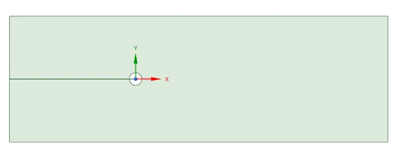
Fig 1 Cylinder and its flow domain

ii) Meshing

First default meshing is done, with element size of 500 mm. Then we will convert the mesh into triangular mesh. Then the edge sizing operation of mesh is performed with number of divisons as 36. The behaviour is soft with no bias type. Then the inflation is done, by selecting the edge of the cylinder, with inflation option as first layer thickness. The first layer height is 5mm with maximum number of layers as 6 and growth rate of 1.2. The inflation is done to obtain the structured mesh so to capture all the fluid variations in the vicinity of the cylinder.

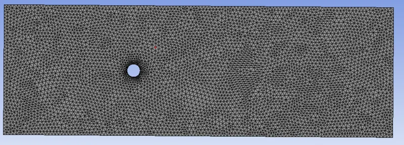
Fig 2 Meshing of cylinder and flow domain

iii) Fluent solver setup

First we have to select the pressure based solver and the steady state condition. Then in model we have to select the laminar model.

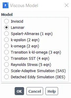
Fig 3 Laminar model selection

In materials we have the air. We will change the density and viscosity values from the default to the new values like 1 kg/m3 and 0.05 kg/ms.

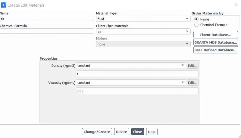
Fig 4 selecting air

Now we come to the boundary conditions. In inlet we give the velocity inlet. We have to calculate the velocity for the corresponding reynolds number. For reynolds number of 10, velocity is 0.25 m/sec.

v = Re (mu) / (rho) D = 10 * 0.05 / 1 * 2 = 0.25 m/sec.

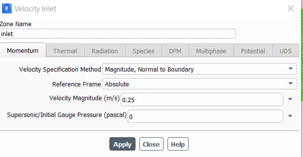
Fig 5 selecting velocity inlet

Now we have to select the pressure outlet.

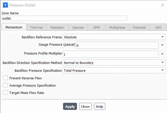
Fig 6 selecting pressure outlet

Now we have to select the reference values.

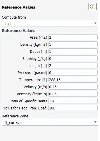
Fig 7 selecting reference values

Now we have to go to solution methods. Here we change the pressure velocity coupling scheme from the default coupled to the SIMPLE scheme. Simple stands for Semi-implicit method for pressure linked equations. This scheme is robust.

Then we create a new point at a distance of 8D from the center of cylinder. We will name this as monitor point.

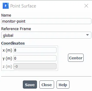
Fig 8 selecting monitor point

Then we will create the report definitions. First for force reports i.e; for drag coefficent and lift coefficient of cylinder wall, then we will create surface report of vertex average velocity at the monitor point.

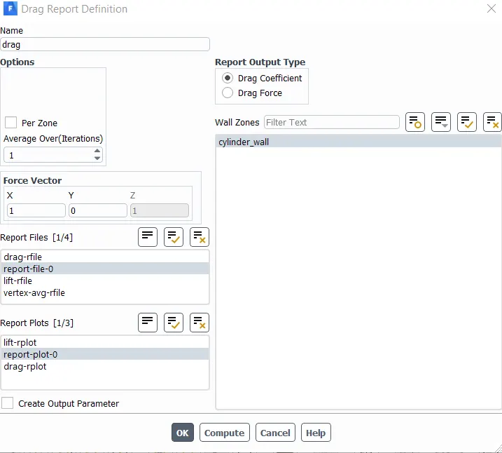
Fig 9 creating drag coefficient report

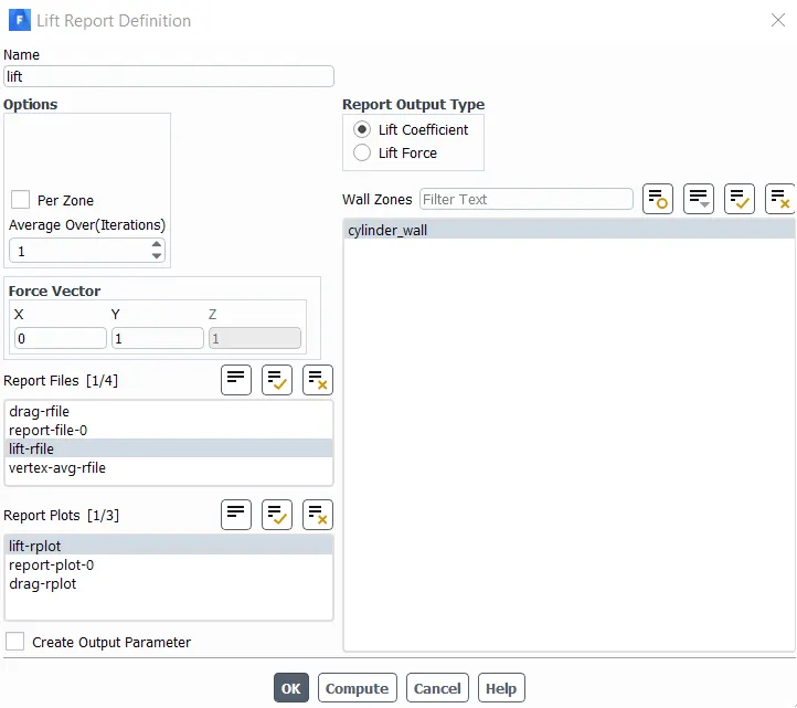
Fig 10 creating lift coefficient report

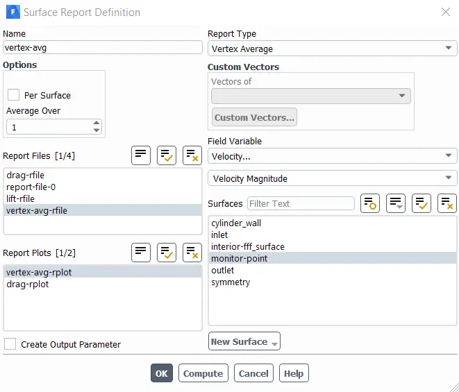
Fig 11 creating vertex average velocity report

Then hybrid initialisation is done and solution is run for 600 iterations.

This is the procedure adopted for running steady case simulation for Re of 10, 100, 1000, 10000 and 100000.

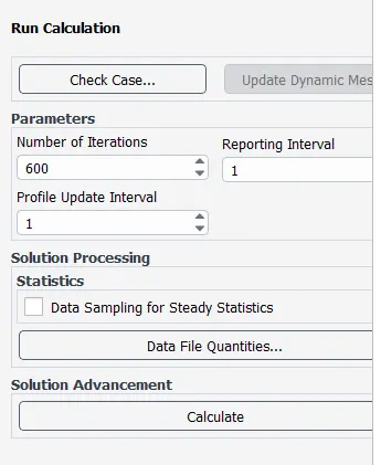
Fig 12 Running iteration in steady case

Now for unsteady simulation for Reynolds number of 10, we have to select transient simulation, and while running calculation we have to mention time step size and number of time steps.

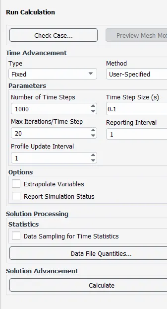
Fig 13 Running iteration in transient case

Fig 13 shows the iterative procedure followed in transient simulation of Re of 10. Time step size of 0.1 sec and number of timesteps of 1000 is used so we will get flow time of 100 sec.

Results:

A. Steady Simulation

(i) Reynolds Number 10

(a) Residual plots

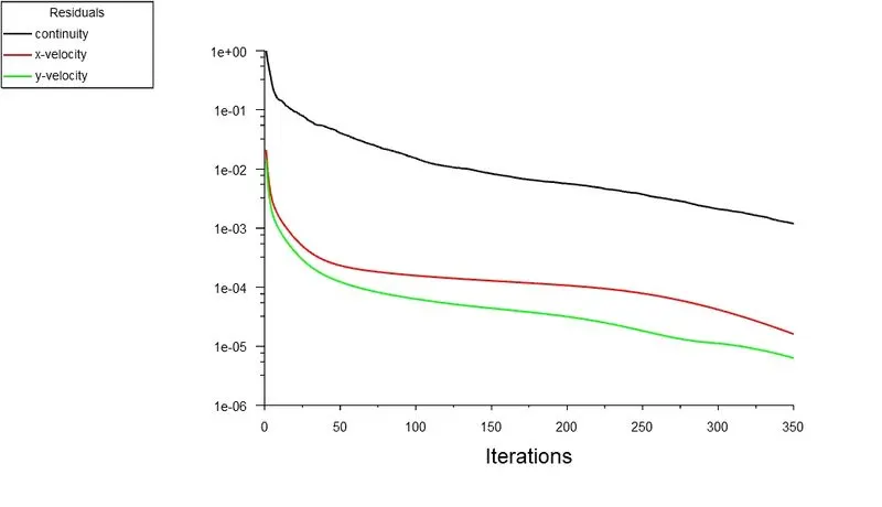
Fig 14 Residual plot

Fig 14 shows the residual plot for Re of 10. The solution attains convergence by running for 350 iterations.

(b) Coefficient of drag

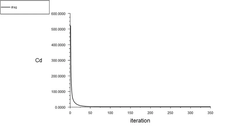
Fig 15 drag coefficient plot

Fig 16 drag coefficient console report

Fig 15 shows the drag coefficient plot while Fig 16 shows drag coefficient around cylinder wall is 3.311.

(c) Coefficient of lift

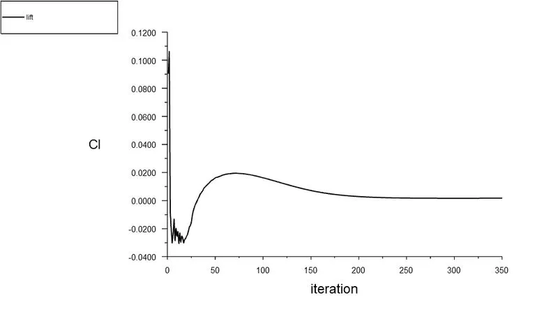
Fig 17 lift coefficient plot

Fig 18 lift coefficient console report

Fig 17 shows the lift coefficient plot while Fig 18 shows its console report value of 0.0017.

(d) Vertex average velocity

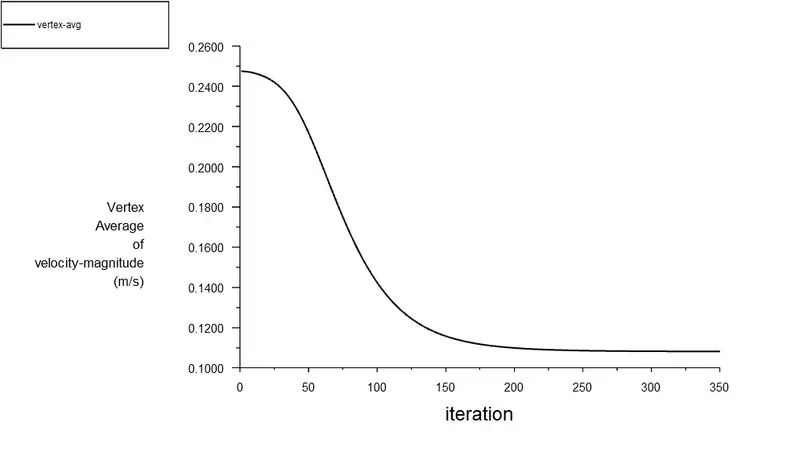
Fig 19 vertex average velocity plot

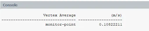
Fig 20 vertex average velocity console report

Fig 19 shows the vertex average velocity plot while Fig 20 shows its console report value of 0.108 m/sec.

(e) Static pressure contour

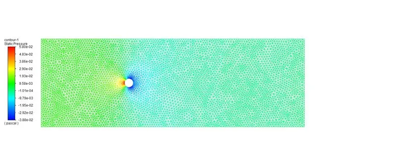
Fig 21 Contour plot of static pressure

Fig 21 shows the static pressure contour plot in the computational domain. Its found static pressure remains higher in the stagnation point, where velocity is zero. The maximum pressure is around 0.058 Pascals.

(e) Velocity contour

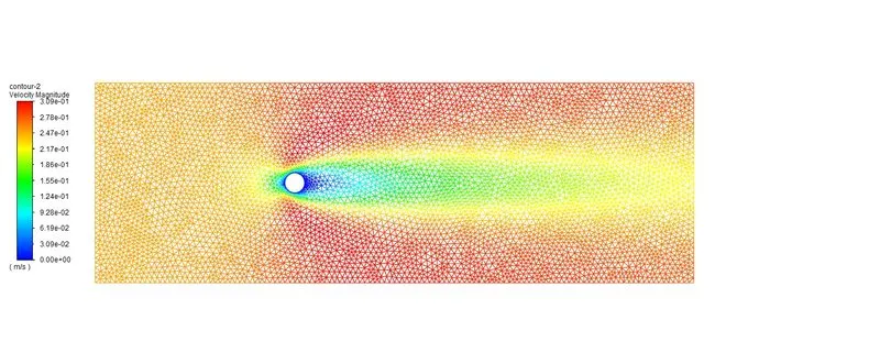
Fig 22 Contour plot of velocity

Fig 22 shows the velocity contour plot in the computational domain. It clearly shows the flow velocity gets decreased in the vicinity of the cylinder, and gets gradually reaching the free stream velocity beyond the boundary layer.

(ii) Reynolds number 100

(a) Residual plots

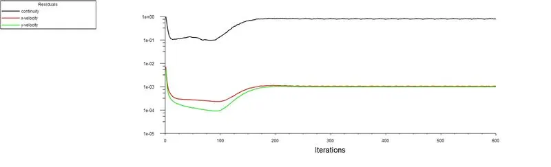
Fig 23 residual plot for Re 100

Fig 23 shows the residual plot for Re of 100. The solution attains convergence by running for 600 iterations.

(b) Coefficient of drag

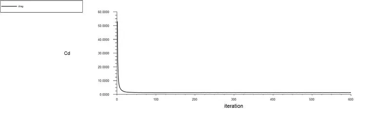
Fig 24 Drag coefficent plot

Fig 25 Drag coefficent console value

Fig 24 shows the drag coefficient plot while Fig 25 shows drag coefficient value around cylinder wall is 1.314.

(c) Coefficient of lift

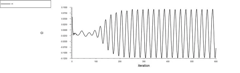
Fig 26 lift coefficent plot

Fig 27 lift coefficent console value

Fig 26 shows the lift coefficient plot while Fig 27 shows lift coefficient value around cylinder wall is -0.079.

(d) Vertex average velocity

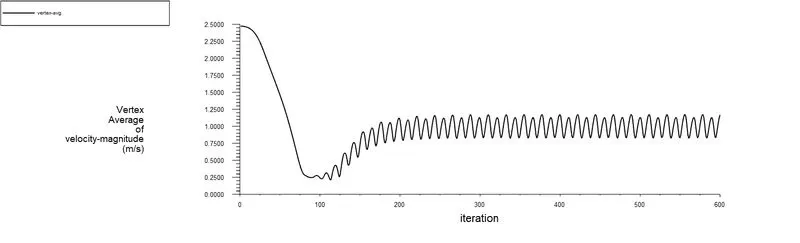
Fig 28 vertex average velocity plot

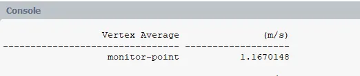
Fig 29 vertex average console value

Fig 28 shows the vertex average velocity of the monitor point at 8m towards right from cylinder center and Fig 29 shows the average vertex console value of 1.167 m/sec.

(e) Static pressure contour

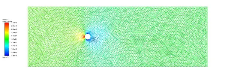
Fig 30 Contour plot of static pressure

Fig 30 shows the static pressure contour plot in the computational domain. Its found static pressure remains higher in the stagnation point, where velocity is zero. The maximum pressure is around 3.7 Pascals.

(f) Velocity contour

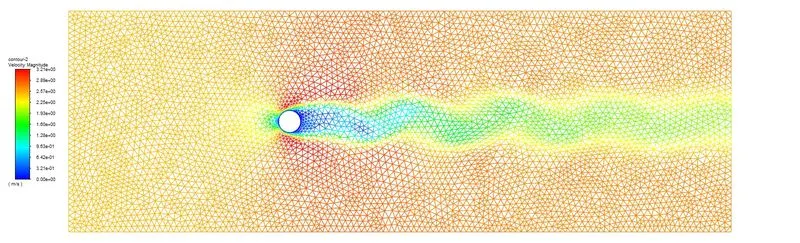
Fig 31 Contour plot of velocity

Fig 31 shows the velocity contour plot in the computational domain. It clearly shows the flow velocity gets decreased in the vicinity of the cylinder, and gets gradually reaching the free stream velocity beyond the boundary layer.

(g) Animation of flow

https://drive.google.com/file/d/17TMDN86RIacruyq2HqoGssd69o7BWstI/view?usp=sharing

(iii) Reynolds number 1000

(a) Residual plots

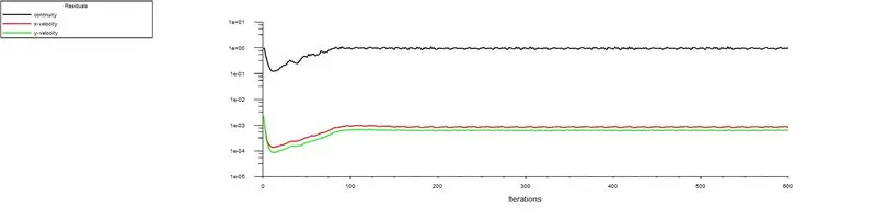
Fig 32 Residual plot for Re 1000

Fig 32 shows the residual plot for Re of 1000. The solution attains convergence by running for 600 iterations.

(b) Coefficient of drag

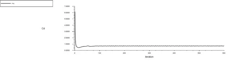
Fig 33 Drag coefficient plot

Fig 34 Drag coefficient console value

Fig 33 shows the drag coefficient plot while Fig 34 shows drag coefficient around cylinder wall is 0.74.

(c) Coefficent of lift

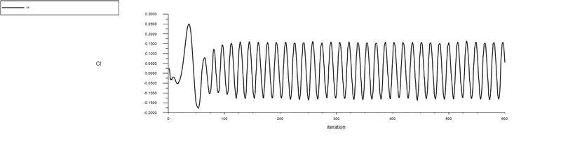
Fig 35 Lift coefficient plot

Fig 36 Lift coefficient console value

Fig 35 shows the lift coefficient plot while Fig 36 shows lift coefficient value around cylinder wall is 0.054.

(d) Vertex average velocity

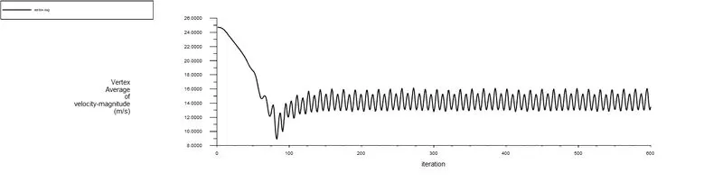
Fig 37 Vertex average velocity plot

Fig 38 Vertex average velocity console value

Fig 37 shows the vertex average velocity of the monitor point at 8m towards right from cylinder center and Fig 38 shows the average vertex console value of 13.47 m/sec.

(e) Static pressure contour

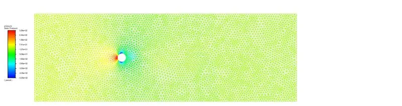
Fig 39 Contour plot of static pressure

Fig 39 shows the static pressure contour plot in the computational domain. Its found static pressure remains higher in the stagnation point, where velocity is zero. The maximum pressure is around 329 pascals.

(f) Velocity contour

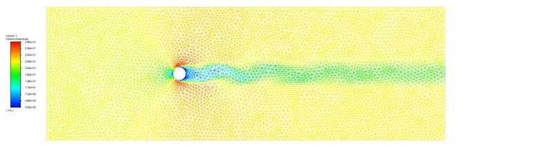
Fig 40 Contour plot of velocity

Fig 40 shows the velocity contour plot in the computational domain. It clearly shows the flow velocity gets decreased in the vicinity of the cylinder, and gets gradually reaching the free stream velocity beyond the boundary layer.

(g) Animation of flow

https://drive.google.com/file/d/1KAOaglmcsrFbn6CFgFUbKKvYUcRotOnJ/view?usp=sharing

(iv) Reynolds number 10000

(a) Residual plots

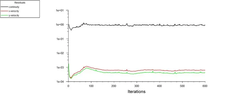
Fig 41 Residual plot for Re 10000

Fig 41 shows the residual plot for Re of 10000. The solution attains convergence by running for 600 iterations.

(b) Coefficient of drag

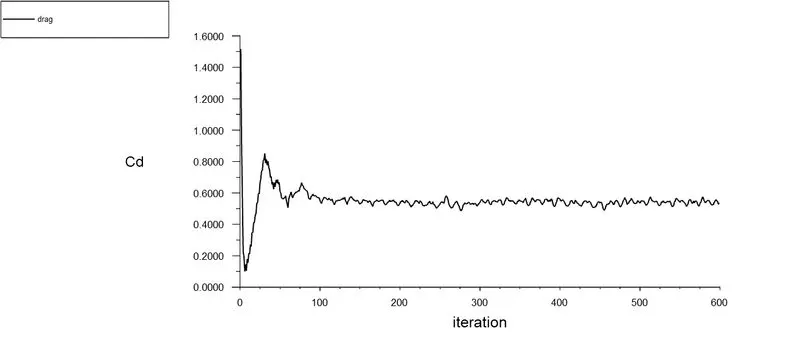
Fig 42 Drag coefficient plot

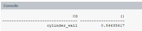
Fig 43 drag coeffiicent console value

Fig 42 shows the drag coefficient plot while Fig 43 shows drag coefficient around cylinder wall is 0.54.

(c) Coefficient of lift

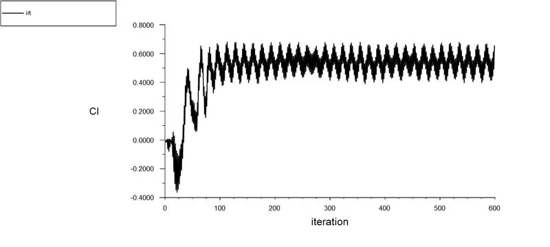
Fig 44 Lift coefficient plot

Fig 45 Lift coefficient console value

Fig 44 shows the lift coefficient plot while Fig 45 shows lift coefficient value around cylinder wall is 0.517.

(d) vertex average velocity

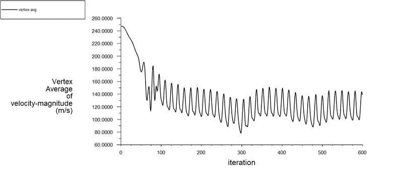
Fig 46 vertex average velocity

Fig 47 vertex average velocity console value

Fig 46 shows the vertex average velocity of the monitor point at 8m towards right from cylinder center and Fig 47 shows the average vertex console value of 129.43 m/sec.

(e) static pressure contour

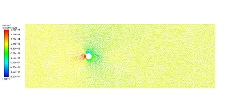
Fig 48 static pressure contour plot

Fig 48 shows the static pressure contour plot in the computational domain. Its found static pressure remains higher in the stagnation point, where velocity is zero. The maximum pressure is around 3080 pascals.

(f) velocity contour

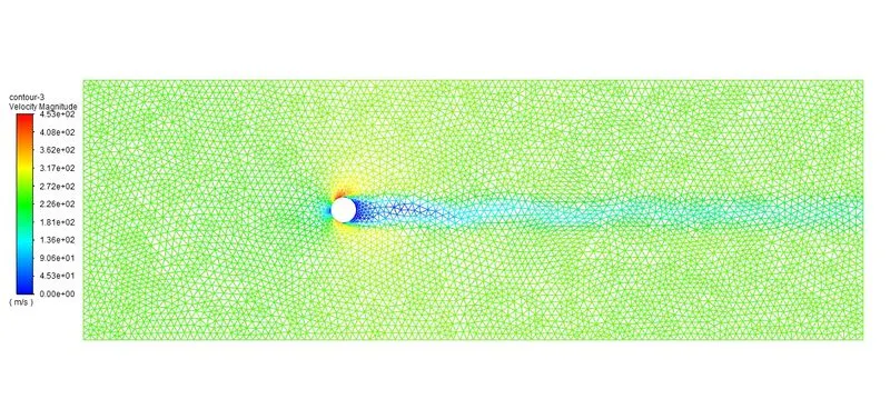
Fig 49 Contour plot of velocity

Fig 49 shows the velocity contour plot in the computational domain. It clearly shows the flow velocity gets decreased in the vicinity of the cylinder, and gets gradually reaching the free stream velocity beyond the boundary layer.

(g) Animation of flow

https://drive.google.com/file/d/13UX2SVGP0X1poqCmR8_5qszQZjI2XuTK/view?usp=sharing

(v) Reynolds number of 100000

(a) Residual plots

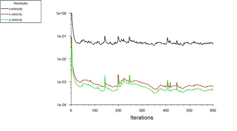
Fig 50 Residual plot for Re 100000

Fig 50 shows the residual plot for Re of 100000. The solution attains convergence by running for 600 iterations.

(b) Coefficient of drag

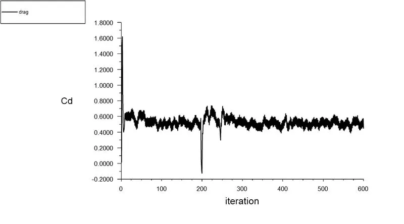
Fig 51 drag coefficient plot

Fig 52 drag coeffiicent console value

Fig 51 shows the drag coefficient plot while Fig 52 shows drag coefficient around cylinder wall is 0.44.

(c) Coefficient of lift

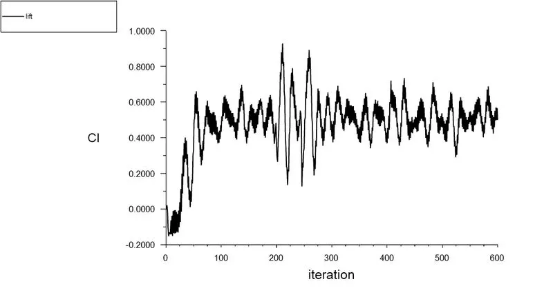
Fig 53 Lift coefficient plot

Fig 54 Lift coefficient console value

Fig 53 shows the lift coefficient plot while Fig 54 shows lift coefficient value around cylinder wall is 0.499.

(d) Vertex average velocity

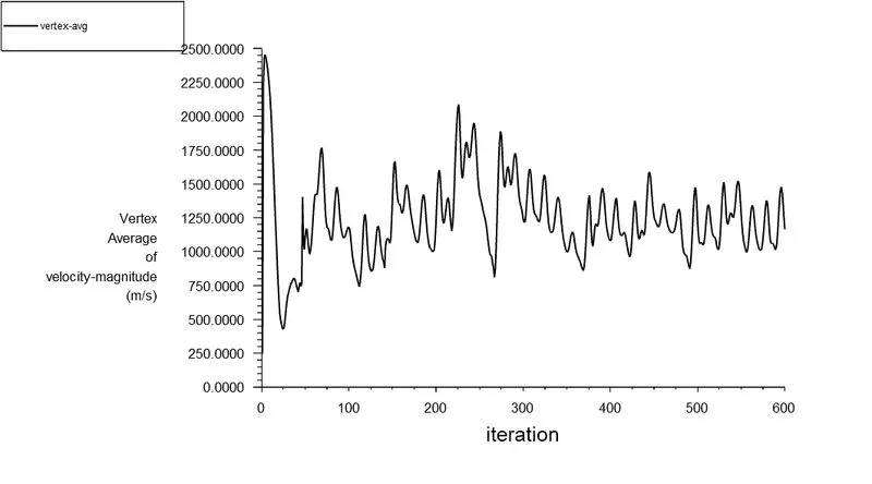
Fig 55 Vertex average velocity plot

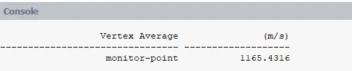
Fig 56 vertex average velocity console value

Fig 55 shows the vertex average velocity of the monitor point at 8m towards right from cylinder center and Fig 56 shows the average vertex console value of 1165.43 m/sec.

(e) static pressure contour

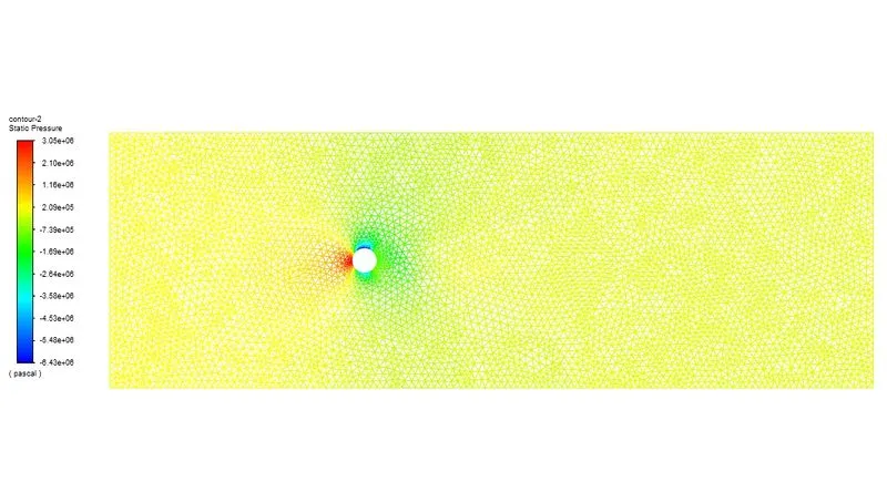
Fig 57 static pressure contour

Fig 57 shows the static pressure contour plot in the computational domain. Its found static pressure remains higher in the stagnation point, where velocity is zero. The maximum pressure is around 3050000 pascals

(f) Velocity contour plot

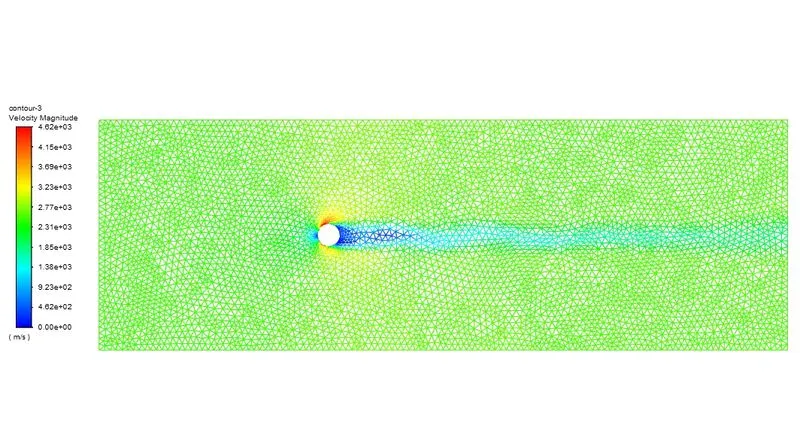
Fig 58 Contour plot of velocity

Fig 58 shows the velocity contour plot in the computational domain. It clearly shows the flow velocity gets decreased in the vicinity of the cylinder, and gets gradually reaching the free stream velocity beyond the boundary layer.

(g) Animation of flow

https://drive.google.com/file/d/13UX2SVGP0X1poqCmR8_5qszQZjI2XuTK/view?usp=sharing

B. Unsteady simulation

(vi) Reynolds number 100

(a) Residual plot

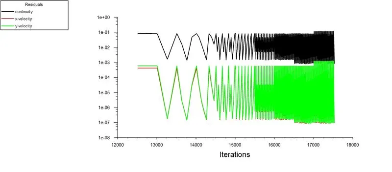
Fig 59 Residual plot for Re no 100 for unsteady flow

Fig 59 shows the residual plots for reynolds number of 100. The residual showing the same pattern for continous iterations hence its infered flow is converged.

(b) Coefficient of drag

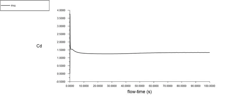
Fig 60 drag coefficient plot

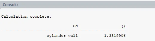
Fig 61 drag coefficient console report

Fig 60 shows the drag coefficient plot while Fig 61 shows drag coefficient around cylinder wall is 1.33.

(c)Coefficient of lift

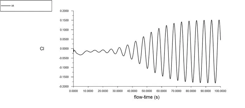
Fig 62 coefficient of lift plot

Fig 63 coefficient of lift console value

Fig 62 shows the lift coefficient plot while Fig 63 shows lift coefficient value around cylinder wall is 0.0449.

(d)Vertex average velocity

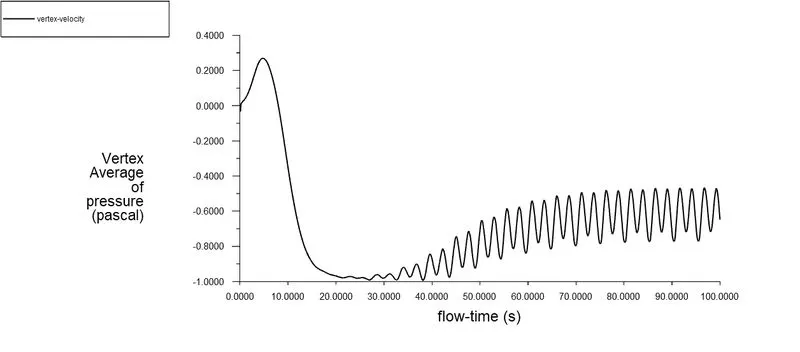
Fig 64 Vertex average of velocity

Fig 65 Vertex average velocity console value

Fig 64 shows the vertex average velocity of the monitor point at 8m towards right from cylinder center and Fig 65 shows the average vertex console value of 1.31 m/sec.

(e) Static pressure contour

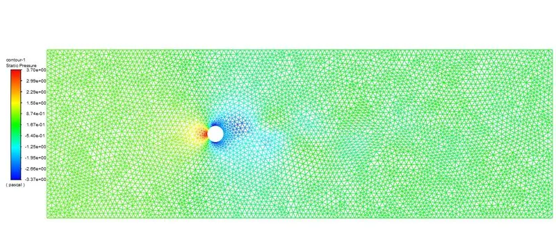
Fig 66 static pressure contour

Fig 66 shows the static pressure contour plot in the computational domain. Its found static pressure remains higher in the stagnation point, where velocity is zero. The maximum pressure is around 3.7 pascals

(f) velocity contour

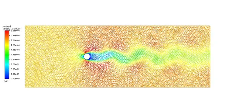
Fig 67 Contour plot of velocity

Fig 67 shows the velocity contour plot in the computational domain. It clearly shows the flow velocity gets decreased in the vicinity of the cylinder, and gets gradually reaching the free stream velocity beyond the boundary layer.

(g) Strouhal number variation

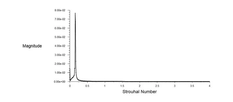
Fig 68 Variation of strouhal number with magnitude

Fig 68 shows the variation of strouhal number with the magnitude and it is found the maximum value is 0.076.

(h) Animation of flow

https://drive.google.com/file/d/1-NTVJ9qSi_LPP0GFv6H3Pe6_9ClogSxd/view?usp=sharing

Conclusions:

Table 1: Variation of parameters with various Reynolds number

S.No	Simulation Type	Reynolds number Re	Drag coefficient Cd	Lift coefficient Cl	Vertex average velocity (m/sec)
1	Steady	10	3.311	0.0017	0.108
2	Steady	100	1.314	0.079	1.167
3	Steady	1000	0.74	0.054	13.47
4	Steady	10000	0.54	0.517	129.43
5	Steady	100000	0.444	0.499	1165.4
6	Unsteady	100	1.33	0.044	1.31

• The above table shows drag coefficient decreases with the increase in the reynolds number, with the maximum coefficient of drag is 3.311 , which is at Reynolds number of 10 and minimum coefficient of drag of 0.444 which is at reynolds number of 100000.
• The video animation shows the vortex shedding occurs at reynolds number of 100 and above 100.
• The vertex average velocity calculated at 8D from center of cylinder , and it shows increasing trend with increasing reynolds number.
• In unsteady simulation we have calculated the strouhal number and the maximum magnitude obtained varying with strouhal number is 0.076.