Week 4 - CHT Analysis on Exhaust port

Aim: To perform conjugate heat transfer simulation on exhaust port using coarser and finer mesh and get the results of average heat transfer coefficient, Wall Y plus, velocity at the outlet, pressure at the outlet and the convection wall average temperature

Introduction: In an IC engine, exhaust manifold or exhaust header is where the exhaust ases will be first collected from the engibe cylinder through exhaust valve. The exhaust gases then further move from the manifold to the catalytic converter then to the muffler etc. Since the exhaust gases will be at very high temperature in the manifold, hence it needs to be very strong. Generally manifolds are made of either cast iron or stainless steel. In an typical gasoline enginethe temperature of hot gases can reach as high as 1000 degree centigrade. So the manifold needs to be thermally stable at high temperature, corrosion resistant etc. There are mainly two types of exhaust manifold: 4 into 1 type and tri y type. Here in our project we are considering 4 into 1 type. We use to give flange support to the pipe inlets, and it needs to be properly welded. Some of the exhaust manifolds used to be coated with ceramics. It acts as a insulator, hence parasitic heat losses can be reduced. So the temperature of the exhaust gases in the manifold will further increase which help in scavenging effect. It will be particularly useful in the turbo engine which generates so much heat, so we can reduce some heat contained in the engine compartment.

Theory:

Conjugate heat transfer corresponds with the combination of heat transfer in the solids and heat transfer in the fluids. In solids, conduction often dominates whereas in the fluids, convection usually dominates. Some of the typical applications are in heaters, heat exchangers and heat sinks. For example shell and tube heat exchangers are used in the thermal power plants as a condenser. The steam from the turbine will be move to the shell side. while cold water from the cooling tower will pass through the tubes in heat exchanger. So here convection heat transfer takes place from the steam to the tube outer surface, conduction takes place through the tube thickness and throughout the tube walls , then again convection takes place from the inner surface of the tube to the cold water; hence heat transfer takes place from the steam to the cold water causing steam temperature to reduce and become saturated water and goes to the pump. In this project, we are considering the exhaust gases from the engine cylinder. Here again we are having the conjugate heat transfer , with convection heat transfer from high temperature exhaust gas to the inside wall of the pipe, then we have conduction heat transfer through the pipe thickness and throughout the pipe, then we have convection heat transfer again from the outer surface of the pipe to the ambient air free stream. In current scenario, where emission norms are strictly followed, proper designing of exhaust systems is important. It also control the noise, vibration and harshness.

Solving and modelling approach:

We will do the modelling in Ansys workbench. We will open the already created model and load in the spaceclaim. First we will do the CAD cleanup, then creating volume extract, then sharing the topology. Then we will do the preprocessing. First we go with the default element size of 150 mm. Then we will perform the inflation layer. Our problem deals with near wall problem, where boundary layer effects are predominant so it is necessary to have fine structured mesh in the vicinity of the wall. So we go with inflation layer, and we will use k omega model is because near wall boundary effect is predominant. Therfore we take y plus value as 10; using Y plus calculator we will calculate the first layer thickness. We get first layer thickness as 0.5 mm, with number of layers as 5. Then we perform inlation layer meshing. Then we will give the necessary named selections. Preprocessing is completed. Now we perform processing using Ansys Fluent solver. We go with the k omega model as already told, then the energy equation on. Then we will check in the cell zone conditions. Then we go with the boundary conditions. For inlet we will give the velocity inlet of 5 m/sec, with the temperature of 700 K, for outlet we give pressure outlet, for convection wall we give heat transfer coefficient of 20 W/m2K with ambient air temperature of 300K. Now in solution methods we give the default COUPLED velocity pressure coupling. Then hybrid intialisation is done and solution is run for 200 iterations. We will obtain the results of average heat transfer coefficient in the inside surface of pipe, temperature distribution in 3 d, pressure, velocity and temperature distribution in XY plane in the outlet pipe. We have also done simulation by varying the base element size to 50 mm, and face sizing of the fluid domain by 10 mm done. Then we obtained the same results and made a comparison with before obtained base mesh element size of 150 mm.

Preprocessing and solver setting:

(i) Geometry creation

First we import the model to the spaceclaim of Ansys Workbench. First we will do ann CAD cleanup if there like removing any unnecessary edges. After that we will add the volume extract to make sure that we have a fluid domain inside. After that we will do the share topology to ensure that the information will be shared correctly between the interface of the exhaust gas and the pipe wall.

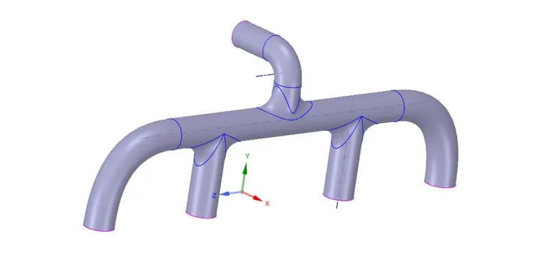
Fig 1 Exhaust manifold geometry

(ii) Meshing

In meshing we use default element size of 150 mm. Then we use inflation layer to capture better wall boundary effect. By using the Y plus calculator we calculated the first layer thickness, it is 0.5 mm. The number of layers is given as 5. Then we will give the named selections : inlet (have 4 inlets), outlet, convection wall and the inflation layer( liquid volume inside)

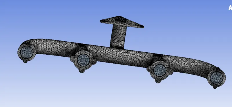
Fig 2 Meshing of Exhaust manifold with base element size of 150mm

Fig 2 shows the meshing of exhaust manifold. We got the number of nodes as 85898 and the number of elements as 243778 respectively.

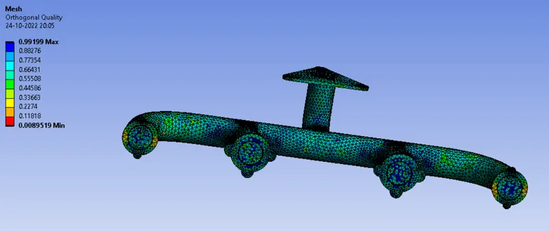
Fig 3 Orthogonal quality check of mesh with base element size of 150mm

Fig 3 shows the orthogonal quality check if mesh. We have got the average orthogonal quality as 0.72 which ensures that mesh is of good quality.

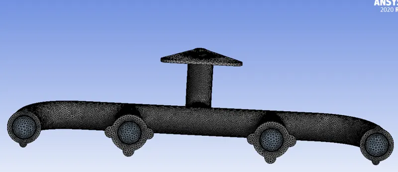
Fig 4 Meshing of Exhaust manifold with base element size of 50mm

Fig 4 shows the meshing of exhaust manifold. We got the number of nodes as 395226 and the number of elements as 1184789 respectively.

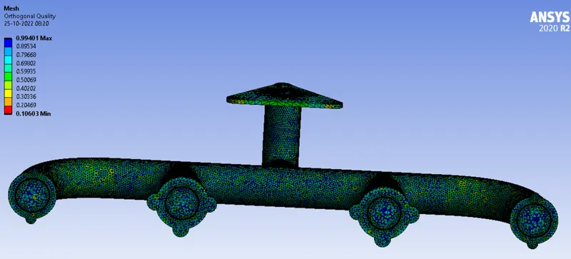
Fig 5 Orthogonal quality check of mesh with base element size of 50mm

Fig 5 shows the orthogonal quality check if mesh. We have got the average orthogonal quality as 0.799 which ensures that mesh is of good quality.

iii) Fluent Solver

First we will enable the steady analysis and the pressure based solver. Then we will enable the models; first energy equation is on since we are dealing with heat transfer in our problem, then we will go with k omega SST turbulence model because we are interested in near wall boundary effects.

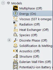
Fig 6 Model selection

After that we will give material selection. We will go with the default air and aluminium.

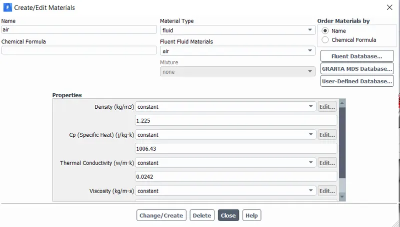
Fig 7 air material selection

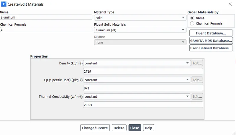
Fig 8 aluminium material selection

Now will go with the boundary conditions. First we will give the velocity inlet boundary conditions. We give the inlet velocity as 5 m/sec and the temperature as 700K.

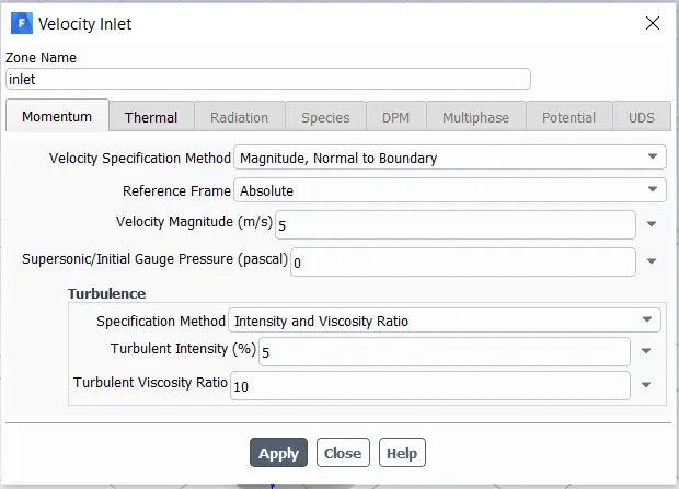
Fig 9 specifying velocity at the inlet

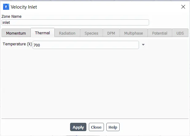
Fig 10 specifying temperature at the inlet

Then we will give the pressure outlet conditions.

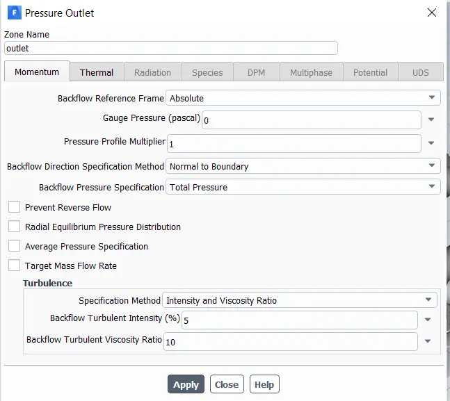
Fig 11 Specifying pressure at the outlet

Then we give the convection wall boundary conditions, specifying the heat transfer coefficient of the air stream at the outlet. The heat transfer coefficient is 20 W/m2K. The free stream temperature is 300K.

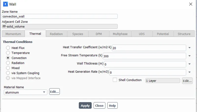
Fig 12 Specifying the heat transfer coefficient at the convection wall

Then in the solution methods we will enable the COUPLED pressure velocity coupling. For momentum, energy, k and omega we will give the default discretization scheme.

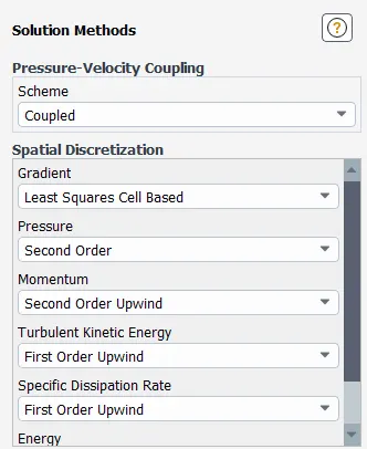
Fig 13 specifying the solution methods

Then we will do the hybrid intialization and the run the solution for 200 iterations.

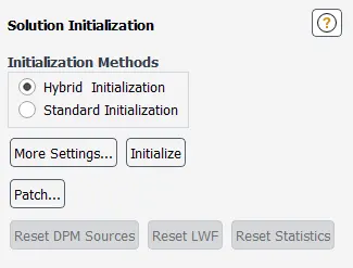
Fig 14 Selecting hybrid intialization

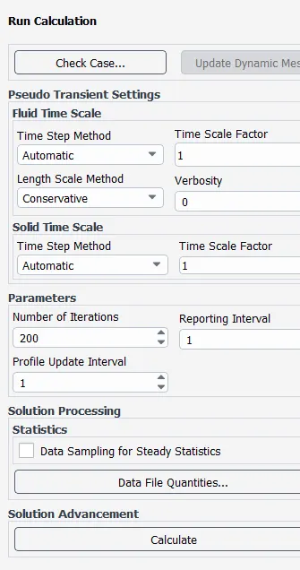
Fig 15 Selecting calculation run setup

Results:

(i) Residuals

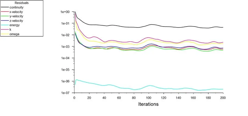
Fig 16 Residual plots for base element size of 150mm

The residuals show the solution is converged by running for 200 iterations.

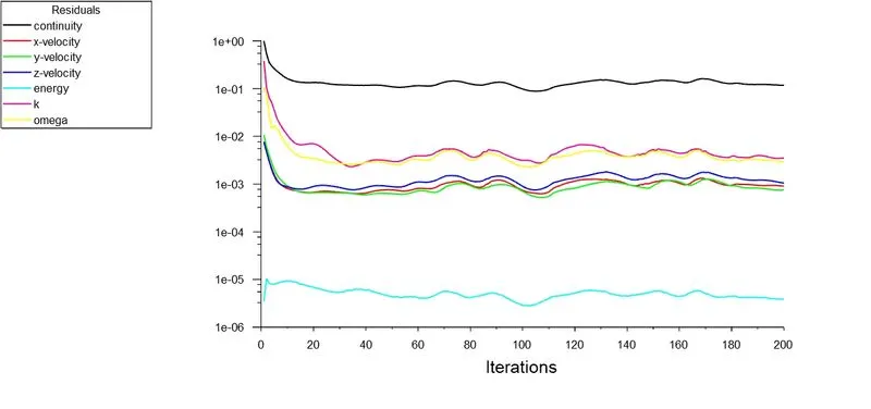
Fig 17 Residual plots for base element size of 50mm

The residuals show the solution is converged by running for 200 iterations.

(ii) Average heat transfer coefficient

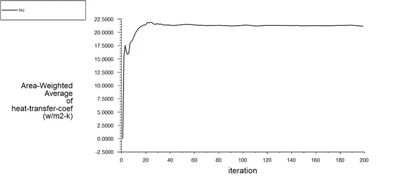
Fig 18 average heat transfer coefficient in the inside surface for base element size of 150mm

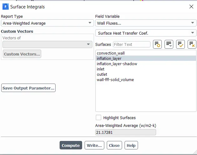
Fig 19 Surface heat transfer coefficient console value for base element size of 150mm

Fig 18 shows the average heat transfer coefficient plots and Fig 19 shows the console report value. We got the area weighted average heat transfer coefficient as 21.17 W/m2K.

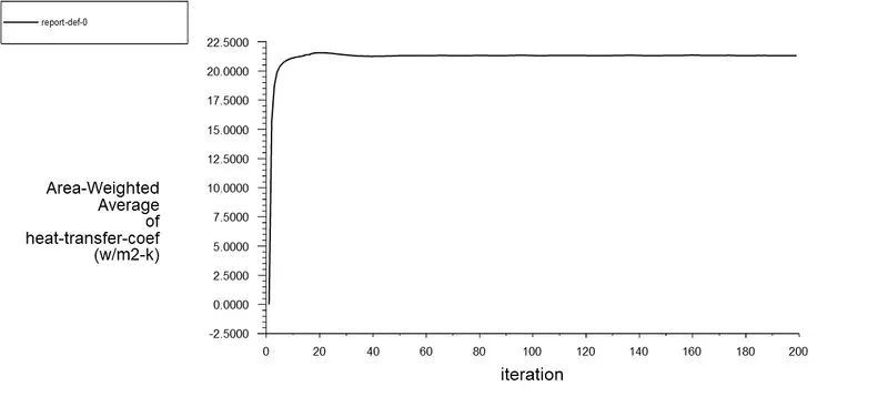
Fig 20 average heat transfer coefficient in the inside surface for base element size of 50mm

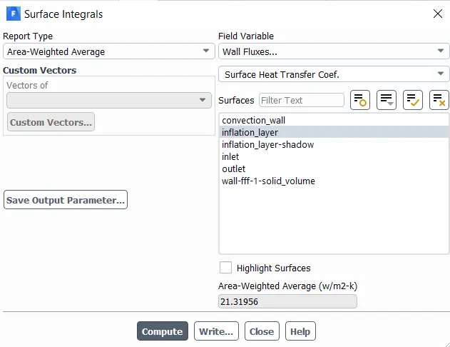
Fig 21 Surface heat transfer coefficient console value for base element size of 50mm

Fig 20 shows the average heat transfer coefficient plots and Fig 21 shows the console report value. We got the area weighted average heat transfer coefficient as 21.31 W/m2K.

(iii) Temperature profile in 3D

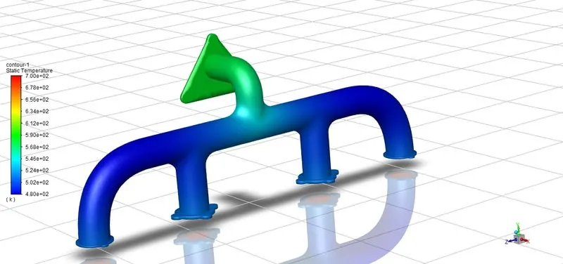
Fig 22 Temperature contour in 3d for base element size of 150 mm

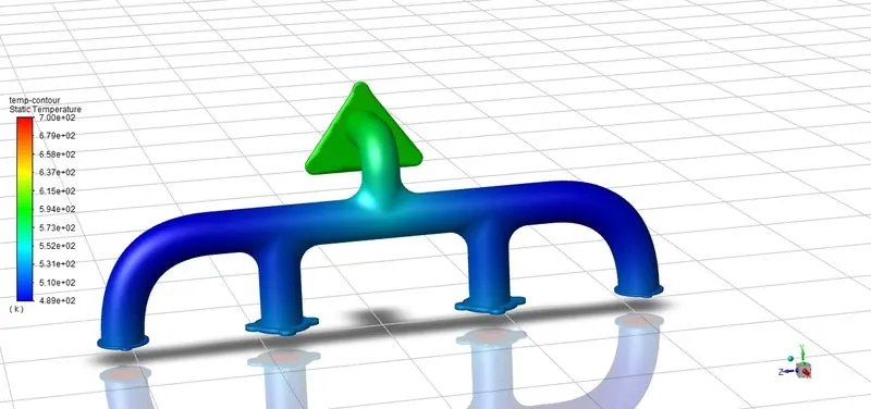
Fig 23 Temperature contour in 3d for base element size of 50 mm

Fig 22m shows the temperature contour in 3d for base element size of 150 mm while Fig 23 shows Temperature contour in 3d for base element size of 50 mm. Its clearly visible there is no distinct difference in the temperature contour profile.

(iv) Pressure contour in XY plane in exhaust port.

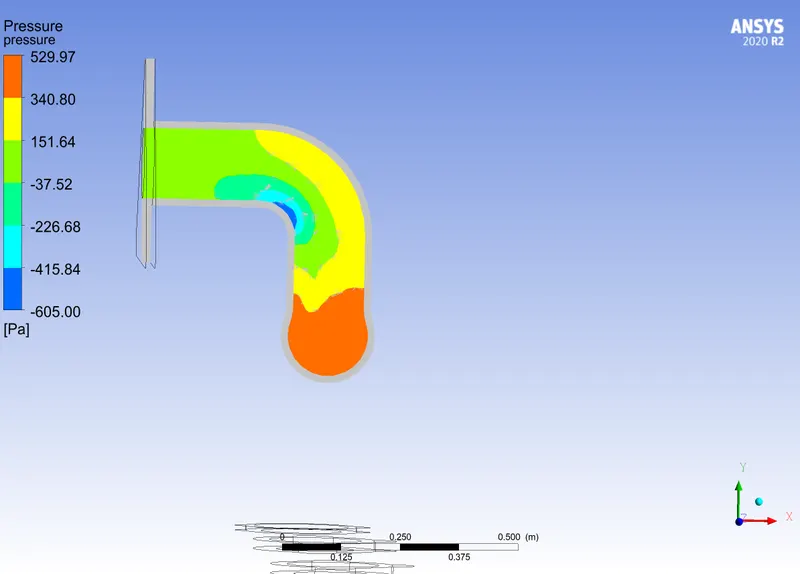
Fig 24 Pressure contour in XY plane in the outlet for base element of 150 mm

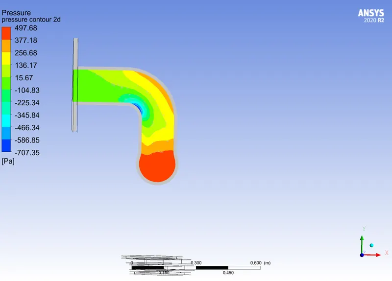
Fig 25 Pressure contour in XY plane in the outlet for base element of 50 mm

Fig 24 shows the Pressure contour in XY plane in the outlet for base element of 150 mm while Fig 25 Pressure contour in XY plane in the outlet for base element of 50 mm. We are seeing pressure maximum at the base point, because its a stagnation point as velocity is zero. Then the pressure shows a drop in value. We can see pressure drops greatly in the pipe bend, and at the outlet again it reaches to atmospheric pressure. We have seen pressure value remains slightly higher in the base element size of 150 mm compared to base element size of 50 mm.

v) Velocity contour in XY plane in exhaust port

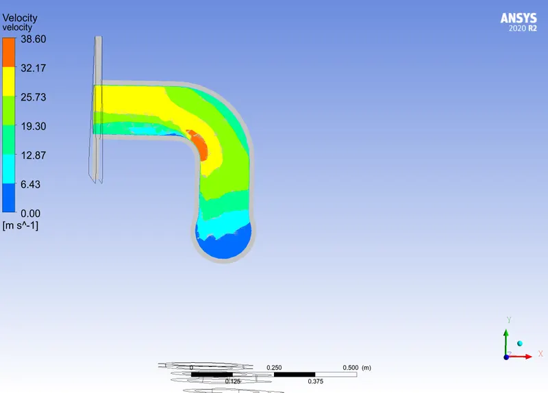
Fig 26 velocity contour in XY plane in the outlet for base element of 150 mm

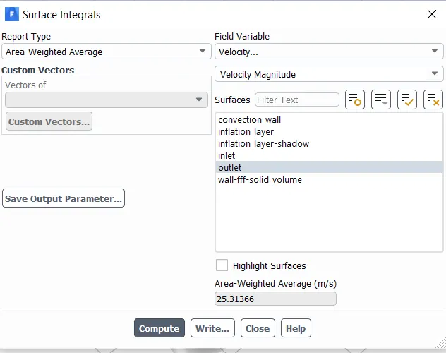
Fig 27 velocity report value in XY plane in the outlet for base element of 150 mm

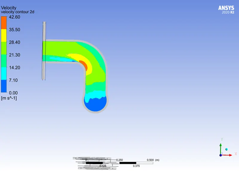
Fig 28 velocity contour in XY plane in the outlet for base element of 50 mm

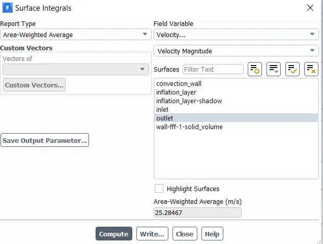
Fig 29 velocity report value in XY plane in the outlet for base element of 50 mm

Fig 26 shows the velocity contour in XY plane in the outlet for base element of 150 mm while Fig 28 shows the velocity contour in XY plane in the outlet for base element of 50 mm. Its clear that the velocity is zero at the bottom part and then gradually increases while exhaust gas moving to outlet. Its clearly seen velocity remains higher in the bend region. From Fig 27 and Fig 29, it is found that the area weighted average velocity at the outlet is 25.31 m/sec and 25.28 m/sec respectively. There is no distinct difference in the velocity values.

vi) Temperature contour in XY plane in exhaust port

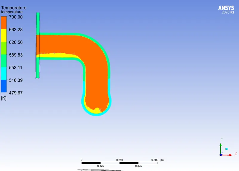
Fig 30 temperature contour in XY plane in the outlet for base element of 150 mm

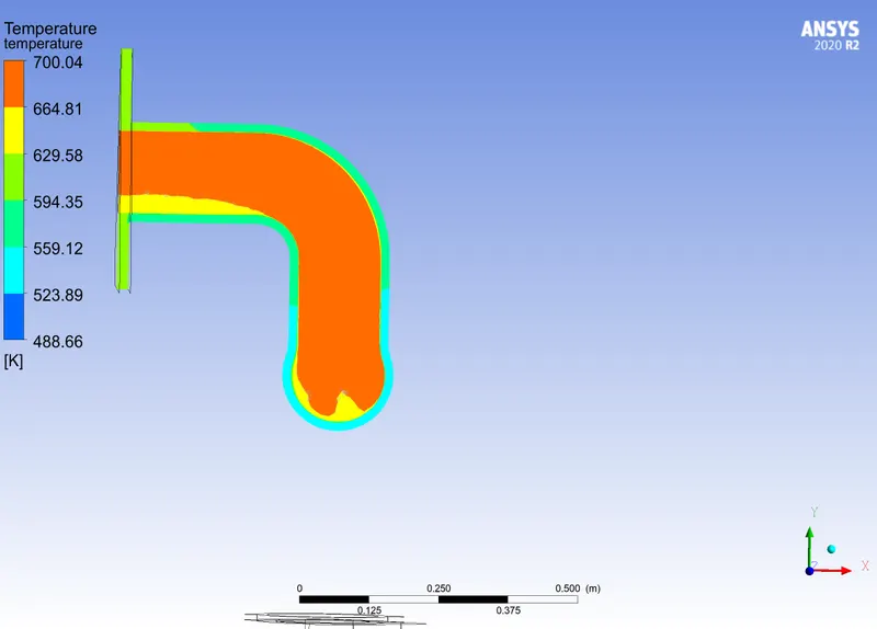
Fig 31 temperature contour in XY plane in the outlet for base element of 50 mm

Fig 30 shows the temperature contour in XY plane in the outlet for base element of 150 mm while Fig 31 shows the temperature contour in XY plane in the outlet for base element of 50 mm. It is observed there is no significant difference in the temperature in both the cases.

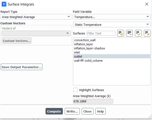
Fig 32 Temperature report value in XY plane in the outlet for base element of 150 mm

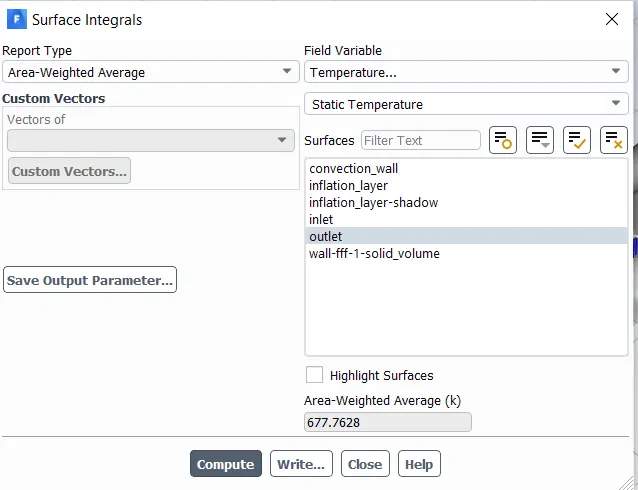
Fig 33 Temperature report value in XY plane in the outlet for base element of 50 mm

Fig 32 Temperature report value in XY plane in the outlet for base element of 150 mm. It shows value is 678.18K. Fig 33 shows Temperature report value in XY plane in the outlet for base element of 50 mm and the value is 677.76K.

vii) Streamlines

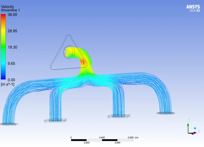
Fig 34 Velocity streamline for base element size of 150mm

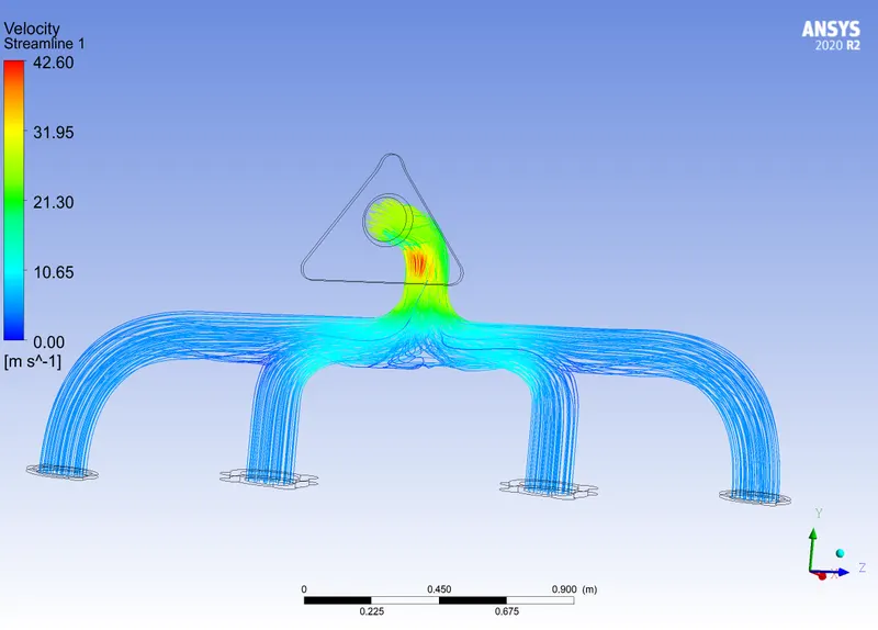
Fig 35 Velocity streamline for base element size of 50mm

Fig 34 shows Velocity streamline for base element size of 150mm while Fig 35 shows Velocity streamline for base element size of 50mm.

Analytical calculation:

Reynolds no. Re = (rho) V D / mu = (1.225 * 5* 0.16 ) / (1.7894 * 10^-5 ) = 54766.96

Now for internal flow in pipe with turbulent flow, we use Dittus Boelter Equation (general equation)

Nu = 0.023 Re^0.8 Pr^0.3 = 0.023 (54766.96^0.8) 0.68^0.3 = 126.55

Nu = hd/k

h = Nu k / d = 126.55 * 0.039 / 0.16 = 30.84 W/m2K.

Conclusions:

Base element size (mm)	No. of elements	Average surface heat transfer coefficient (W/m2K)	Outlet velocity (m/sec)	Outlet temperature (K)	Turbulence wall Y plus
150	243778	21.17	25.31	678.18	7.523
50	1184789	21.31	25.28	677.76	7.97

• We have performed simulation on an exhaust port using two different base element sizes of 150 mm and 50mm. We have found that there is no significant differences in the results obtained as shown in the table above.
• Since we have considered near wall boundary effects we have used k omega turbulence model, and in calculation of first layer thickness we have used y plus value of 10. The simulation results showed turbulence wall Y plus value of 7.523 in base element size of 150mm and 7.97 in the base element size of 50mm. There is no much difference.
• The analytical calculation is also made of heat transfer coefficient and there is less difference between experiment and simulation results.