Week 5 - Rayleigh Taylor Instability

Aim: To perform Rayleigh Taylor instability simulation for water and air multiphase system for two different mesh sizes ( coarse and fine ) and make a comparison of the results; similarly run the simulation for water and user defined material.

Introduction: Rayleigh Taylor instability is the instability of interface between two fluids of different densities when the lighter fluid pushes the heavier fluids. In fluid dynamics it comes under the field of hydrodynamic stability where we will study about stability and instability of fluid flows. It is the instability created by density stratification. So what happens is because of the density difference , the two fluids will try to reduce their combined potential energy. When the lighter fluid is above the denser fluid the system is stable but when the denser fluid is above lighter fluid , there will be unstable interface between the two fluids and the lighter fluid slowly pushes up and equal volume of denser fluid moves down. Then the potential energy is now lower than the intial state and the disturbance will grow, leads to turbulence.

Theory: Rayleigh Taylor instability finds its application in both natural and man made phenomena. Some examples are overturn of outer portion of collapsed core of massive star, formation of high luminiosity twin exhaust jets in rotatting gas clouds in external gravitational field. Some of the technological applications are laser implosion of deuterim tritium fusion targets, electromagnetic implosion of metal liners. Some of the practical CFD models of Rayleigh taylor instability are water lying on top of oil in gravity field, explosion of atom bombs causing gases to rise up forming mushroom clouds.

If we consider the simulation the water lying on oil surface in the Ansys Fluent, since it is a multiphase simulation we have to enable it. There are various multiphase models available , here we consider VOF model (volume of fluid) . It is mostly advisable to perform transient analysis than steady state analysis so that the flow fluctuations can be captured perfectly for small time scales , with selecting low timestep size values. One of the feature of VOF model is that all the cells must be filled with atleast one fluid before performing simulation. We can take care of this by performing patching of phases after intialisation. This can initialise the initial condition. In VOF analysis we can perform either implicit or explicit method. If we perform explicit method, then courant number plays a major role. It needs to be less than 1, so that all the flow doesnt miss any cell or control volume during simulation and also for better solution stability. If we perform implicit method, then no need to give courant number. In this case , we consider implicit scheme. Similarly while running calculation, we can either give fixed or adaptive time step calculating method. In fixed, time stepsize remains constant while in adaptive, time stepsize (sec) automatically readjusts to ensure that the courant number is less than 1, hence flow is not converged.

Solving and modelling approach:

First the model is created in the spaceclaim of Fluent from Ansys Workbench. First the air domain is created, then the water domain. Then the surface of both created , then the shared topology is done. Then the preprocessing is done, for the first case with the coarse mesh, element size being 0.5mm , then for the second case with fine mesh, with element size being 0.1mm. Then we have to ensure the mesh is of fine quality by checking the aspect ratio and orthogonal quality. thus the preprocessing is done, then we go for processing. Now we go for processing in fluent solver. First we enable transient analysis since we want to capture the interface instabilities in small timescales, then we enable gravity with y = -9.8 m/s2. It is a laminar model. Since we are not considering any heat transfer in this simulation energy model is not enabled. Then we have to use multiphase model with vof model (Volume of fluid). Here we have to give phase details, primary phase being air and secondary phase being water. Then in methods we go with the default SIMPLE pressure velocity coupling.

Here we havent change anything with respect to reference values. Then we go for intialisation. Here we use hybrid initialisation , and then patching of the phases are done. Here volume fraction patching is done, with volume fraction of water given 1 in the water surface, and volume fraction of water is given 0 in the air surface. Then we run for iterations. we will give the number of timesteps and the time stepsize (sec). For element base size of 0.5 mm we used timestep size of 0.01 sec and 500 number of timesteps with number of iterations per timestep being 20. So this gives flowtime of 5 seconds. But while running iteration for element size of 0.1mm, with timestep size of 0.01 sec and 500 timesteps, it showed divergence in the continuity equation at 324th iteration. Then i gradually reduced the timestep size from 0.01 sec to 0.005 sec with 500 number of timesteps, then also divergence was observed at 825th iteration. Therefore, finally i selected timestepsize of 0.001 sec with 2500 timestepsize and got the results. Then the animation file of volume fraction of water phase is created. After that we will perform simulation of water and user defined material multiphase system and obtained animation file of volume fraction of water using the above same procedure.

Preprocessing and solver settings:

(i) Geometry creation

First we open Ansys workbench, then we will select the fluent module. Then we will select the spaceclaim option and create the model. Then we will create a rectangle of 20mm by 20 mm. Then we will create surface by using return to 3d mode option. Then we will name the component as air. After that we will create another rectangle, which is at top of the air surface and its dimensions are 20 mm by 20 mm, again creating surface by using return to 3d mode option, then we will create the component as water. After that we will perform the share topology so that it will share the interface.

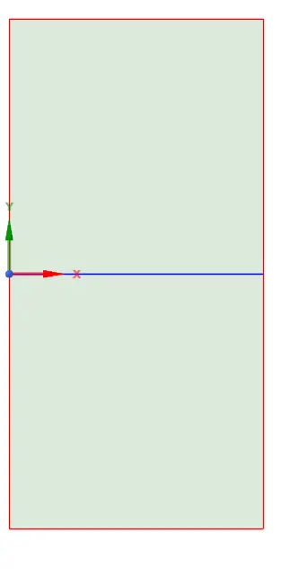
Fig 1 : Geometry of water and air

(ii) Mesh creation

Mesh is created with element size of 0.5mm. Then we got the number of nodes as 3321 and number of elements as 3200 respectively.

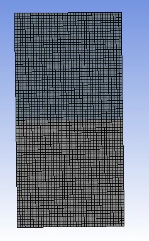
Fig 2 : Mesh generated (element size 0.5mm)

Then the mesh quality is checked. For this we use orthogonal quality check. We got the average orthogonal quality value as near to 1, hence mesh quality is good.

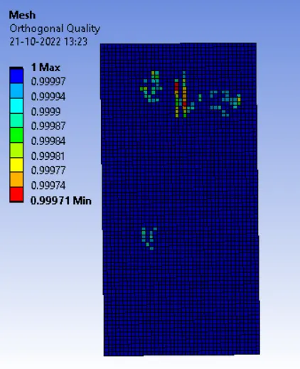
Fig 3 : Orthogonal quality check of mesh (element size 0.5mm)

For the next case to get more fine mesh, we performed meshing with element size of 0.1mm. Then we got the number of nodes as 80601 and number of elelments as 80000 respectively.

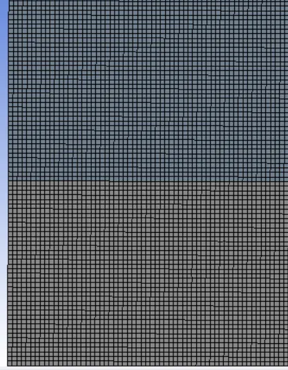
Fig 4 : Mesh generated (element size 0.1mm)

Since it was not able to capture the mesh of entire geometry clearly while taking picture, just 40 percent of the geometry is shown above.

Then the mesh quality is checked. For this we use orthogonal quality check. We got the average orthogonal quality value as near to 1, hence mesh quality is good.

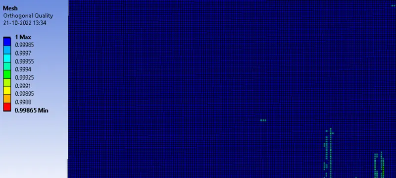
Fig 5 : Orthogonal quality check of mesh (element size 0.1mm)

(iii) Fluent setup

In fluent setup first we have to enable the transient time analysis and enable the gravity.

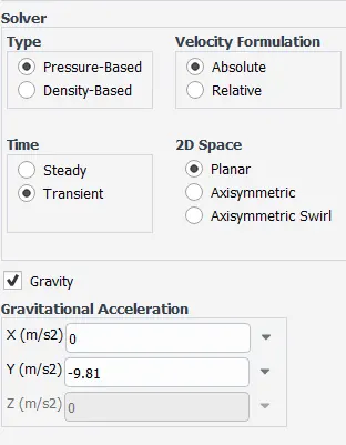
Fig 6 : Enabling transient analysis and gravity

In models we will consider laminar model, and multiphase models with volume of fluid enabled.

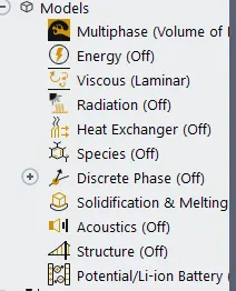
Fig 7. Selecting the models.

While enabling vof model, we have to give the phase names, primary phase being air, and secondary phase being water liquid; and we will enable implicit formulation in volume fraction parameters.

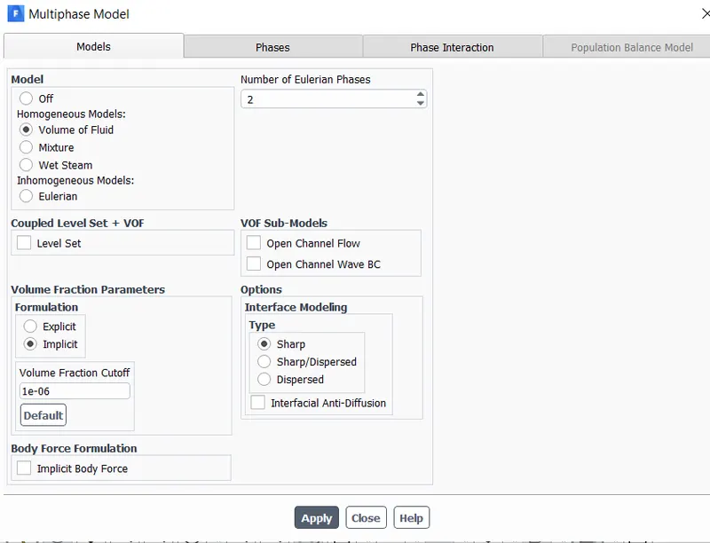
Fig 8 Selecting the multiphase vof model

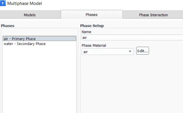
Fig 9 Selecting the phases in vof model

In solution methods, we enable the SIMPLE pressure-velocity coupling; with PRESTO pressure discretization, second order upwind discretization for momentum and compressive scheme for volume fraction.

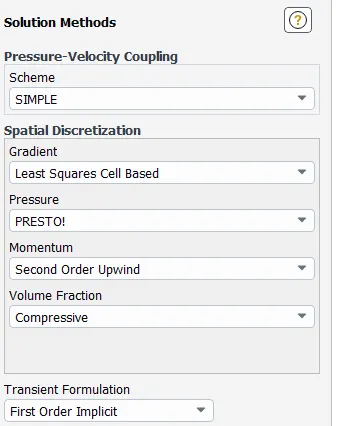
Fig 10 Selecting the solution methods

For solution intialization, we perform hybrid intialisation with patching of volume fraction of phases. The volume fraction of water being 1 in water surface and volume fraction of water being 0 in the air surface.

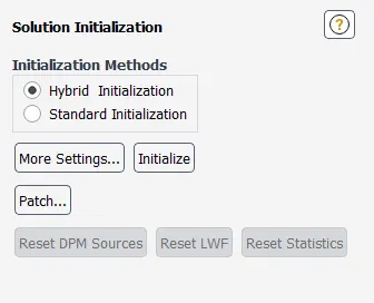
Fig 11 Solution intialization

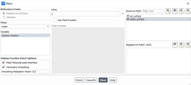
Fig 12 Patching of volume fraction of water as 1 in the water surface

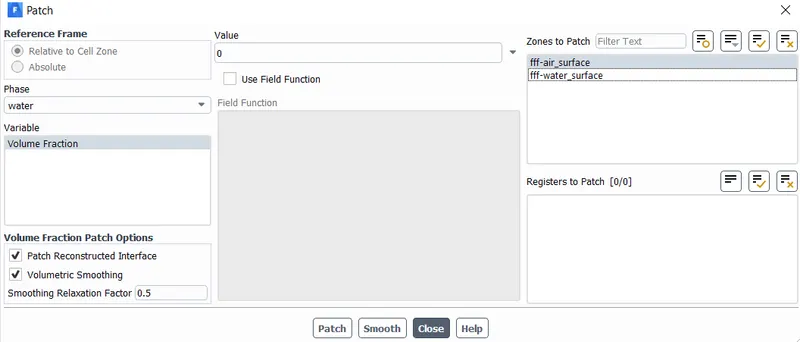
Fig 13 Patching of volume fraction of water as 0 in the air surface

Now we will run the calculation. Since this being transient simulation, we have to give timestep size(sec) and number of timesteps. For element size of 0.5mm, we give 0.1 sec as timestepsize and 5000 as number of timesteps. For element size of 0.1mm, we give 0.01 sec as timestepsize and 2500 as number of timesteps.

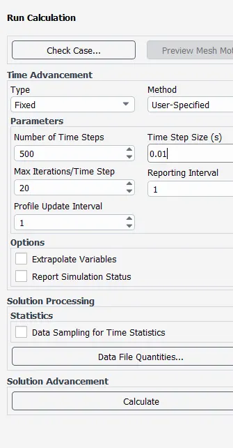
Fig 14 Calculation setup for 0.5 elementsize

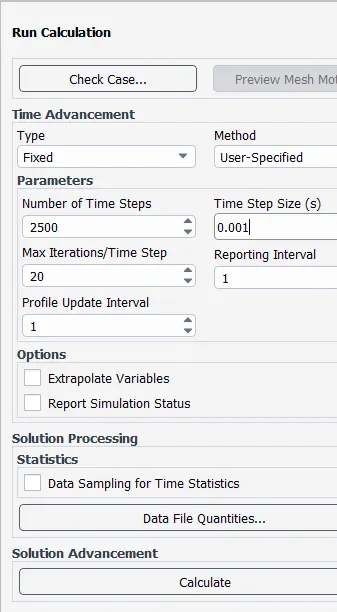
Fig 15 Calculation setup for 0.1 elementsize

Similarly we have done calculation for water and user defined material (density 400 kg/m3 and viscosity 0.001 kg/ms).

The mesh we used is same of 0.1 element size as before. The number of timesteps and timestep size are also of the same value of 2500 and 0.001 sec respectively.

Results:

(i) Residuals

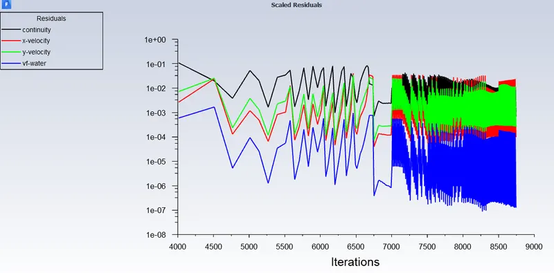
Fig 16 Residual plots for element size of 0.5mm

Fig 16 shows the repeating pattern of the residuals which implies the solution has converged.

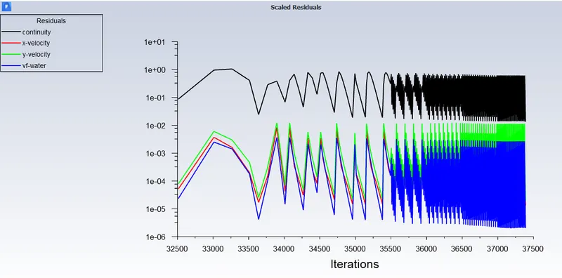
Fig 17 Residual plots for element size of 0.1mm

Fig 17 shows the repeating pattern of the residuals which implies the solution has converged.

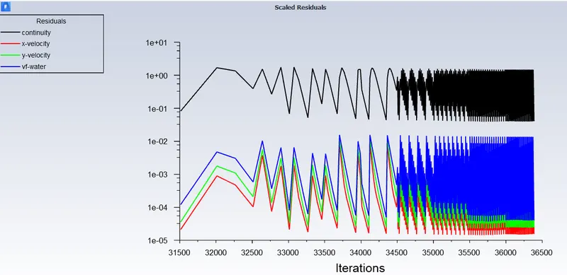
Fig 18 Residual plots for element size of 0.1mm for water and userdefined material multiphase system

Fig 18 shows the repeating pattern of the residuals which implies the solution has converged.

ii) Animation videos

a) Animation video of volume fraction of water in water air multiphase system at 0.5 mesh element size

https://drive.google.com/file/d/12mlGxjP0XHrLC4rqsp1U6b3HafKUqsgc/view?usp=sharing

b) Animation video of volume fraction of water in water air multiphase system at 0.1 mesh element size

https://drive.google.com/file/d/1mMdgpqfLF_zymwaWpXw0wyCWo5tWX9Ek/view?usp=sharing

We can make a comparison between the animation of water air system for two different mesh sizes, one coarser mesh and other finer mesh. We find that we are able to capture larger fluctuactions in the eddies formation in the finer mesh compared to the coarser mesh. Therefore more accurate solution is obtained in the finer mesh but one disadvantage is the higher computational time and hence the higher computational cost.

The steady state simulation is not suitable for this kind, because we need to have very small timescales to capture all the fluid disturbances and fluctuations which is not possible in steady simulation and also in transient simulation we can control the timestep size so we can capture the disturbances based on the value given; we also have to ensure courant number wont exceed 1.

c)Animation video of volume fraction of water in water user defined material multiphase system at 0.1 mesh element size

https://drive.google.com/file/d/114KQiABNgw_x2T497BcK-YeelMNEE5UQ/view?usp=sharing

Atwood number is a dimensionless number which is used in the fluid dynamics to study about hydrodynamic instabilities in density stratified flows. It is denoted by the letter A and is given by

A =( rho 1 - rho 2 ) / (rho 1 + rho 2 )

where rho 1 is the density of heavier fluid an

and rho 2 is the density of lighter fluid

For water air multiphase system,

Atwood number A = (1000 - 1.225) / (1000 + 1.225 ) = 0.9975

For water user defined material multiphase system,

Atwood number A = (1000 - 400 ) / (1000 + 400 ) = 0.428

We have observed that the atwood number of air water multiphase system is higher than the atwood number of water-userdefinedmaterial multiphase system. Higher atwood number implies the interface can achieve stability bit faster compared to lower atwood number.

Conclusions:

We have done simulation of air water multiphase system with coarse mesh as well as fine mesh and a comparison is made such that we were able to capture more flow disturbances across the phase interface in the fine mesh model compared to coarse mesh model. We have discussed why transient simulation is important in vof model compared to steady simulation. Then we made a comparison between water air multiphase system and water userdefined material multiphase system; Atwood number was used a parameter to make the comparison and it was discussed that that the higher Atwood number in the air water system (0.9975) helps it to achieve interface stability faster compared to lower Atwood number (0.428) in the water userdefined material multiphase system.