Week 1- Mixing Tee

Aim: To determine the mixing effectiveness as well as the outlet temperature and outlet velocity of the air in the mixing tee problem. Here four cases are considered:

Case1: Short Tee with momentum ratio of 2

Case 2: Short Tee with momentum ratio of 4

Case 3: Long Tee with momentum ratio of 2

Case 4: Long Tee with momentum ratio of 4

Momentum ratio is the ratio of velocity of cold air at inlet to the velocity of hot air at inlet.

Introduction:

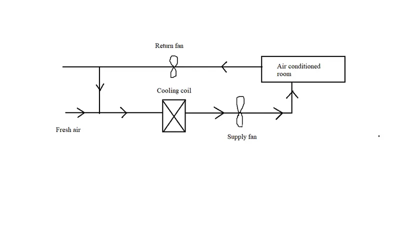
The mixing of air streams is having its main applications in the HVAC industry. The mixing of fresh air with the recirculated air from the air conditioned room is used to provide necessary ventilated space in the buildings and other residential places. This can control the amount of fresh air used carefully. This can increase the efficiency of the system. The diagram below shows the application of air mixing system in HVAC system

Theory:

There is a need for proper ventilation and conditioning of air inside buildings to make sure the occupants are getting sufficient air at all the conditions. This ensures we are getting sufficient oxygen from the air, and after we are exhaling we are releasing carbon dioxide which needs to be vented out. The accumulation of carbon dioxide in the room can cause health problems hence proper monitoring of its concentration should be there. A typical home will have 1 or 1.5 tonne air conditioner with R 22 or R 32 as refrigerant. This is generally used in single room, where number of occupants will be less say 2 or 3. Therefore, there is no need to supply additional fresh air supply. But, if we consider central air conditioning in malls, hospitals etc the number of occupants will be very high. Therefore additional supply of fresh air is mandatory. For this, there will be some ducts for air passage. In certain applications inorder to optimise the usage of fresh air judiciously we can mix the fresh air with the recirculated air coming from the air conditioned room. The mixed air then passes through the cooling coil and from there to the air conditioned room. Then the exhaust air from the room is recirculated back into the intake system with the help of return fan. The optimised design of intake fresh air duct system as well as recirculated air duct system is necessary to achieve desired performance. The CFD tool can be used here, to study the streamline of flow, the pressure, velocity and temperature distribution for various geometric design parameters and we can select a particular geometric size where performance wise as well as cost wise is in balanced state.

Solving and modelling Approach:

The 3 D model of short tee and long tee is imported to the Spaceclaim field of Ansys Workbench. The hot air inlet flow is in positive X direction, while the cold air inlet flow is in negative Y direction and the outlet mixture flow is in positive X direction. Since we are concerned only with the fluid physics and there is no heat transfer phenomena through the pipe wall, we can suppress the solid wall and consider only the fluid part for solving. The imported geometry doesnt have fluid region inside threfore we have to generate fluid flow inside using the following commands: Prepare and volume extract. We have to select the inside edges of hot air inlet pipe, cold air inlet pipe and outlet pipe and generate volume. After this we have compressed the solid shell for physics. Now the model is ready for preprocessing. In preprocessing, we will divide the fluid domain into large number of control volumes (elements) so that we can compute the parameters like pressure, velocity and temperature inside it. Since this is a fluid domain, number of elements will be much larger than the number of nodes. The navier stokes equation ( Conservation of mass, momentum and energy equations) have to be solved through this elements. Since this partial differential equations will be difficult to sove we have to discretize it into algebraic form using various numerical methods. Based on the problem used we have to use various solver schemes for momentum, energy and pressure. After mesh is generated we can see whether the mesh generated is of good quality using orthogonal quality check, skeweness check etc. Then using statistics we can check the number of elemetns and nodes created and based on the qaulity of mesh generated we can either stick with the generated mesh for further processing or we can modify the mesh using various options like face sizing, edge sizing , inflation etc. After this named selections have to be given, which will be used later in the boundary conditions in the fluent solver. Here named selelctions are given for inlet, outlet and the wall. After this we can click on update mesh and close the mesh and open the setup from the Workbench. This will open the Fluent solver. Then we have to select the model associated with our problem. That is we have to select whether flow in the computational domain is laminar or turbulent, if its turbulent again we have to select whether it is k omega model or k epsilon model depending upon the flow physics. Then we have to assign the materials, which will be available in the fluent database. Incase the material is not available in the fluent database we can create the material and assign its properties. Then the cell zone conditions will be coming, here we have to assign whether its fluid or solid and its operating conditions. Then the boundary conditions we have to assign. It can be inlet condition, wall condition and outlet condition. For inlet we can consider, velocity-inlet, mass flow rate-inlet, pressure-inlet etc. For outlet also we can follow the same. For wall we have to give condition depending on whether heat flux is present or not. Then we have to give reference values; here we will compute from inlet and reference zone also needs to be mentioned. For methods we will follow the default values. Then we will do the intialization. After that we will create report plots for average temperature at the outlet and standard deviation of the temperature at outlet. Then we will run for 600 iterations and check whether convergence is met.The default convergence criteria is used here. Then we will get the residual plots and report plots. Then we can close setup and open Solution from workbench. Then we will get 3D contour plots of temperature and velocity distribution. Then we will get the average value of temperature results in the console by going to the reports, then to surface integrals and then selecting weighted average temperature etc. Then we will close the solution and open the results from the workbench. In results first we will create new plane 1, which is in XY direction. Then we will obtain the contours of velocity, temperature and velocity vector in XY plane. Then we will create chart. For this first we have to create new line which is the centerline and then create temperature chart which is a graph between temperature on the Y axis and X (length) on the X axis. Similarly new velocity chart also created which is a grapph between velocity on the Y axis and X(length) on the X axis.

Preprocessing and solver setting:

i) Geometry creation

Here two geometries are considered: one is short Tee and other is Long Tee.

a) Short Tee

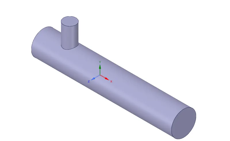
Fig 1 Geometry of Short Tee

Hot fluid inlet diameter = Outlet fluid diameter = 33.9 mm

Cold fluid inlet diameter = 17 mm

Length of pipe = 192.4 mm

b) Long Tee

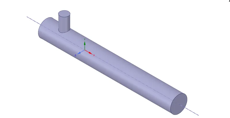
Fig 2 Geometry of long Tee

Hot fluid inlet diameter = Outlet fluid diameter = 33.9 mm

Cold fluid inlet diameter = 17 mm

Length of pipe = 268.32 mm

The geometries have been imported into the spaceclaim module of Ansys Workbench. For the first case we will consider the short tee.Then first we will fill the pipe with fluid domain. For that first we will go to prepare ribbon button and click on volume extract, then we will select the inner diameter edges of hot inlet pipe, cold inlet pipe and outlet pipe. Then we will generate the volume. Then we will suppress the solid shell as it is not interfering in the physics of the problem, Then we will measure all the required dimensions using measure ribbon and calculate diameters of hot inlet pipe, cold inlet pipe and length of pipe. Then we will save the project close the spaceclaim window and open the mesh frrom workbench.

ii) Mesh creation

First we heve to go to mesh details and go to basic element size. We will select basic element size of 3 mm. Then we will enable inflation with five layers with a growth rate of 0.2.

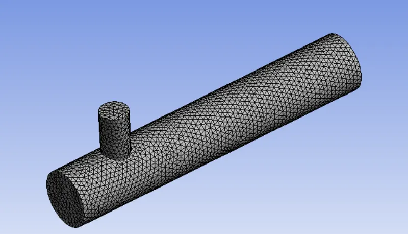
Fig 3 Mesh generation on short Tee

Fig 3 shows the mesh generated on the short Tee. The number of elements and nodes created are 39879 and 8369 respectively.

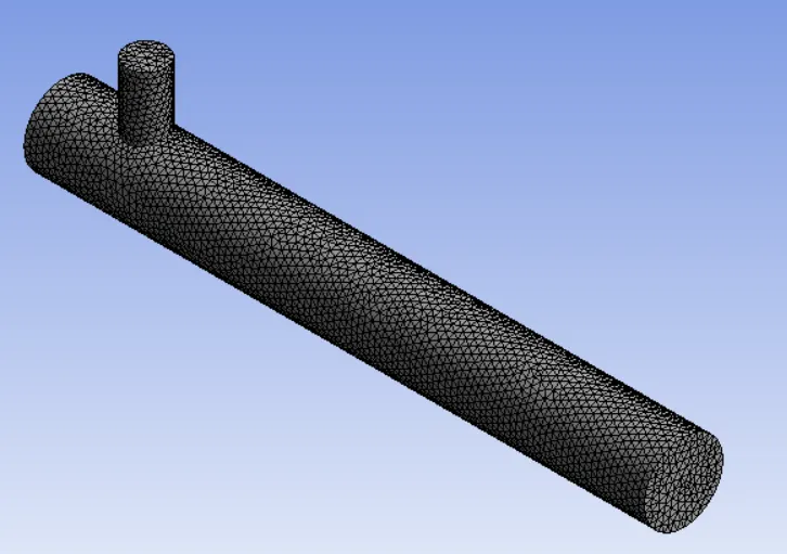
Fig 4 Mesh generation on Long Tee

Fig 4 shows the mesh generated on the Long Tee. The number of elements and nodes created are 56504 and 11710 respectively.

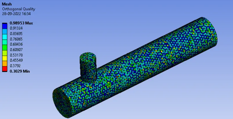
Fig 4 Othogonal quality of mesh on short Tee

Fig 4 shows the orthogonal quality of mesh generated on short tee. The desired value is approximately near to 1 and we got a satisfactory mesh.

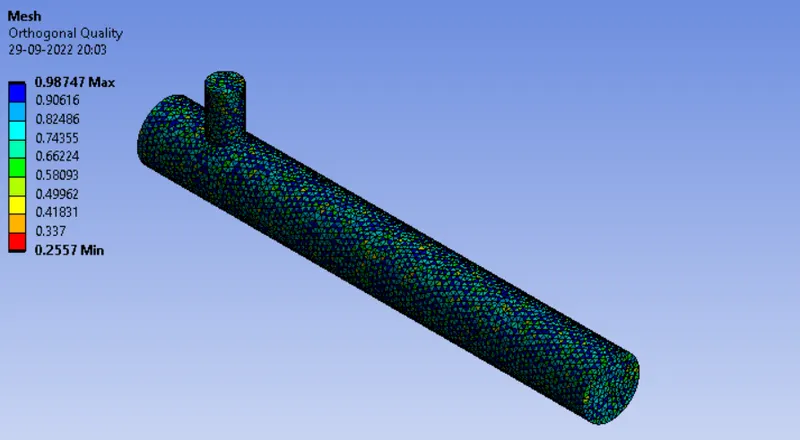
Fig 5 Othogonal quality of mesh on Long Tee

Fig 5 shows the orthogonal quality of mesh generated on long tee. The desired value is approximately near to 1 and we got a satisfactory mesh.

iii) Setup of Fluent Solver

First in general option we will enable pressure based solver and time as steady time.

In models we will enable k- epsilon model with standard wall functions. We will enable energy equation on

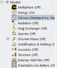
Fig 6 Model selection

In materials for fluid we will consider air. By default air is selected in ansys fluent.

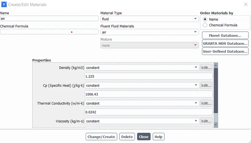
Fig 7 Fluid material selection

Now we will proceed with boundary condition. ie. a) inlet b) outlet

a) Inlet

First is Inlet x

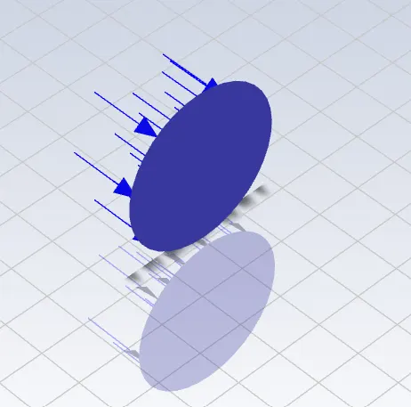
Fig 8 Hot fluid inlet flow in x direction

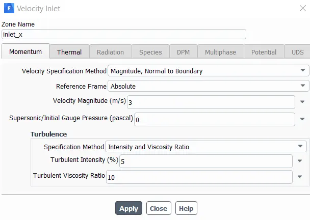
Fig 9 Hot fluid Inlet X velocity specification

Fig 9 shows the hot air velocity of 3 m/s specified in the x direction.

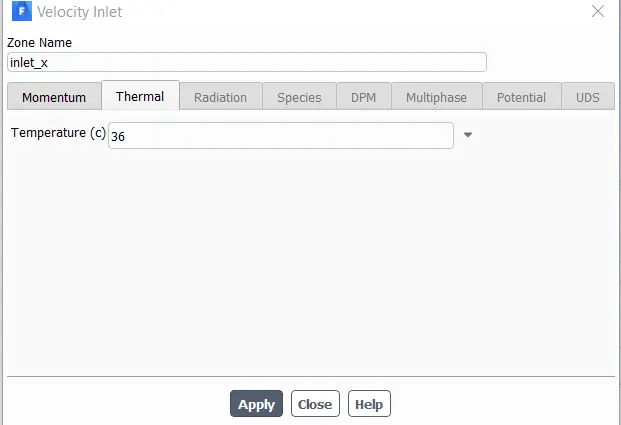
Fig 10 Hot fluid Inlet x temperature specification

Fig 10 shows the temperature specification of the hot air inlet in the x direction.

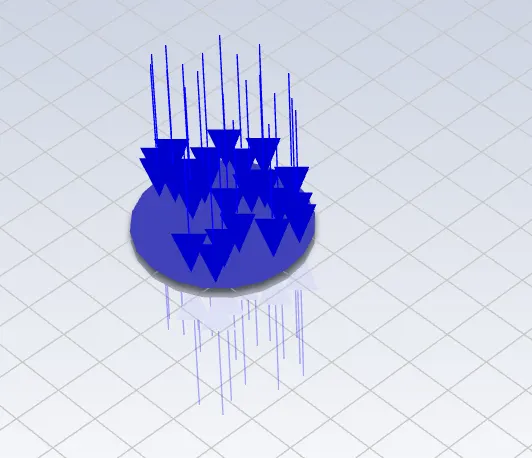
Fig 11 cold fluid inlet flow in y direction

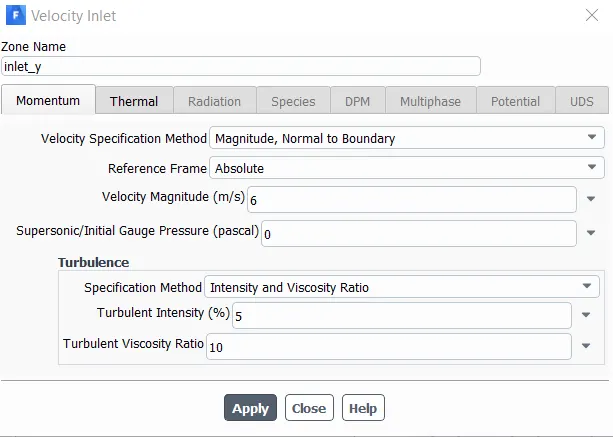
Fig 12 Cold fluid inlet velocity specification

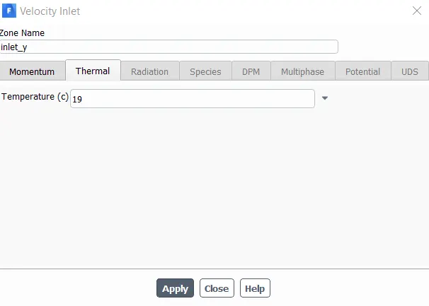
Fig 13 Cold fluid Inlet y temperature specification

b) Outlet

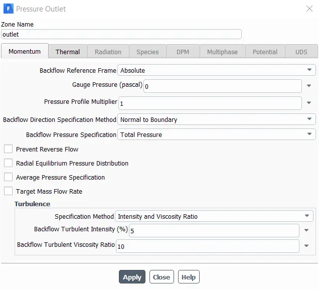
Fig 14 Mixed fluid pressure outlet

Now we will give the reference values to perform the computation

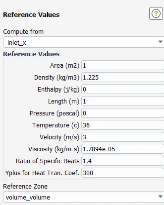
Fig 15 Reference values specification

Fig 15 shows the specification of reference values. We will perform computation from inlet x.

In solution methods we will follow the default values.

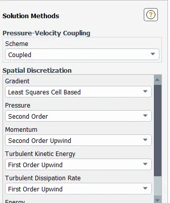
Fig 16 Solution methods specification

Now in report definitions we will create new report plots from the surface reports. First we will create area weighted average of temperature at outlet and next we will create standard mean deviation of outlet temperature.

After this we will perform the solution intialisation with hybrid intialisation and then we will run the calculation for 600 iterations.

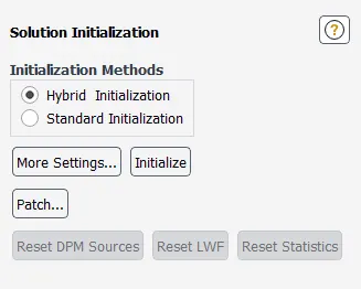
Fig 17 Solution intialisation specification

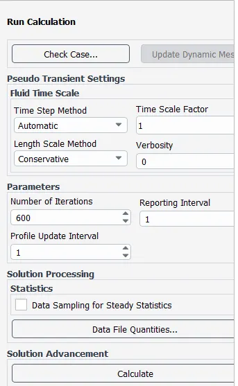
Fig 17 Run calculation specification

Results:

(i) Residual plots

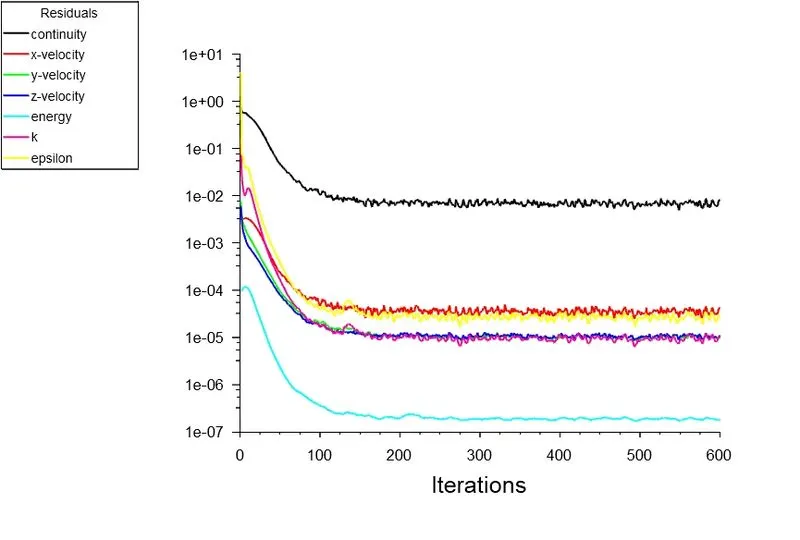
Fig 18 Residual plot for Short Tee (M.R=2)

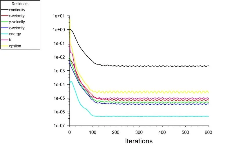
Fig 19 Residual plot for Short Tee (M.R=4)

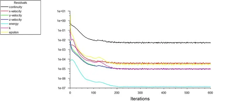
Fig 20 Residual plot for Long Tee (M.R=2)

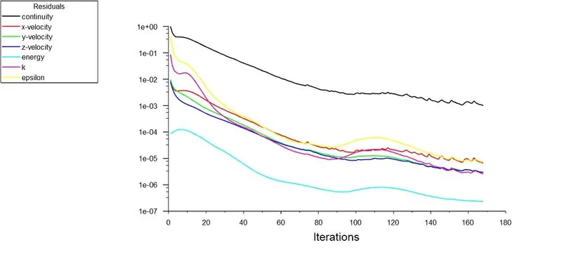
Fig 21 Residual plot for LongTee (M.R=4)

Fig 18, Fig 19, Fig 20 and Fig 21 shows the residual plots for the Short Tee( M.R = 2), Short tee (M.R = 4), Long Tee (M.R =2) and Long Tee (M.R = 4) respectively. We have run the calculation for 600 iterations for all the cases. We got the converged solution in all the cases. In 4th case the solution got converged at 168th iteration only.

ii) 3D Contour plot of Temperature and Velocity distribution.

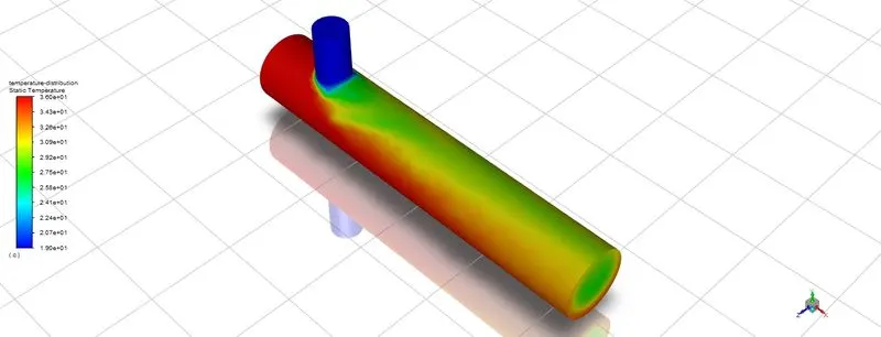
Fig 22 Contour plot for Temperature for short tee (M.R=2)

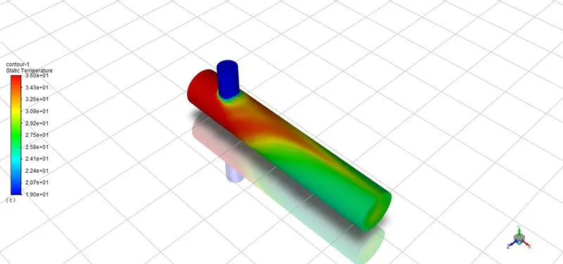
Fig 23 Contour plot for Temperature for short tee (M.R=4)

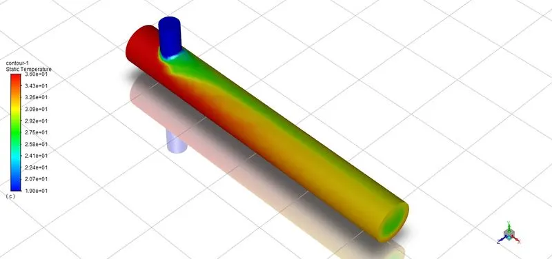
Fig 24 Contour plot for Temperature for long tee (M.R=2)

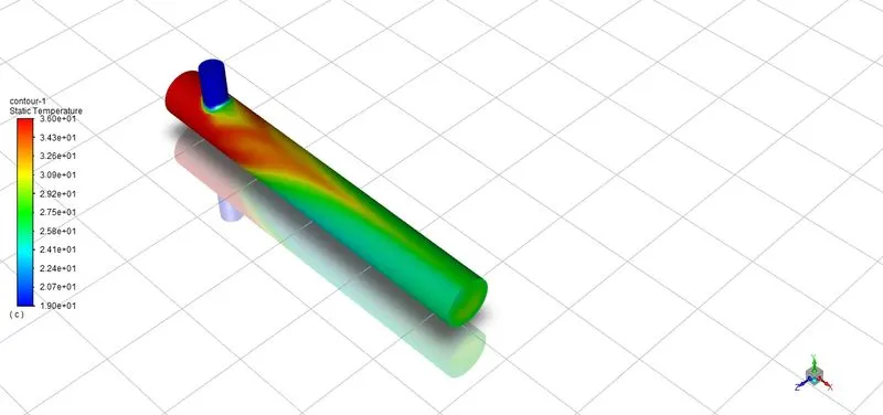
Fig 25 Contour plot for Temperature for long tee (M.R=4)

Fig 22, Fig 23, Fig 24 and Fig 25 shows the temperature distribution of fluid flow for short tee (M.R=2), for short tee (M.R = 4), Long Tee (M.R =2) and Long Tee (M.R=4) respectively. The contour plots clearly shows that the overall temperature distribution remains higher for M.R = 2 compared to M.R=4 for both short tee and Long Tee.

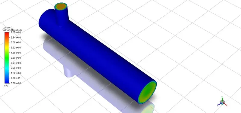
Fig 26 Contour plot for velocity for short tee (M.R=2)

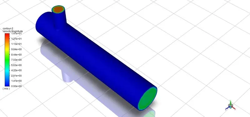
Fig 27 Contour plot for velocity for short tee (M.R=4)

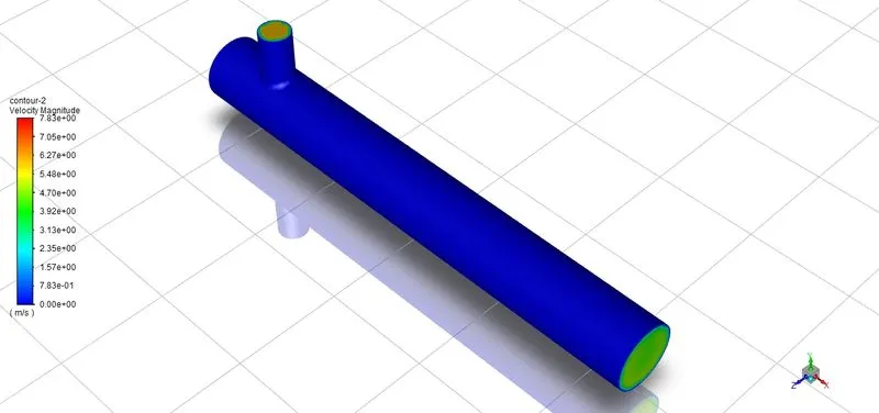
Fig 28 Contour plot for velocity for long tee (M.R=2)

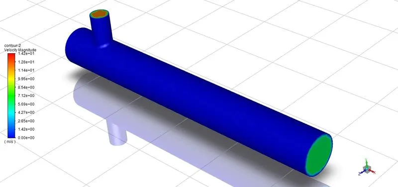
Fig 29 Contour plot for velocity for long tee (M.R=4)

Fig 26, Fig 27, Fig 28 and Fig 29 shows the velocity distribution of fluid flow for short tee (M.R=2), for short tee (M.R = 4), Long Tee (M.R =2) and Long Tee (M.R=4) respectively. From the contours it is understood that the velocity distribution throughout the fluid domain remains higher for M.R = 4 than M.R= 2 . This is because of higher velocity of cold fluid of 12 m/sec in the case of M.R = 4 compared to 6 m/sec in the case of M.R = 2.

iii) 2 D contour plot of Temperature, velocity and velocity vector in XY plane

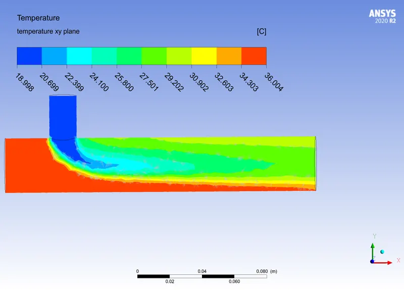
Fig 30 Contour plot for temperature in XY plane for short tee (M.R=2)

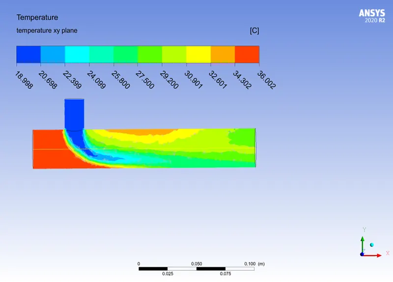
Fig 31 Contour plot for temperature in XY plane for short tee (M.R=4)

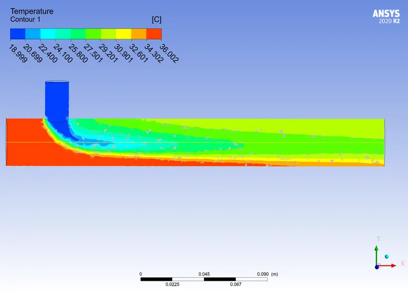
Fig 32 Contour plot for temperature in XY plane for long tee (M.R=2)

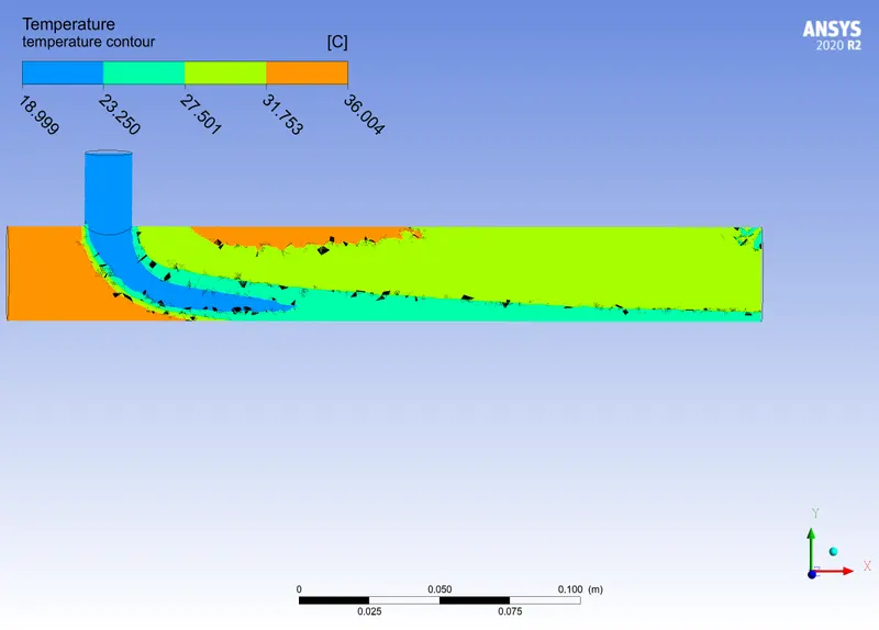
Fig 33 Contour plot for temperature in XY plane for long tee (M.R=4)

Fig 30, Fig 31, Fig 32 and Fig 33 shows the temperature profile in XY plane for all the four cases respectively. It is found that for short tee (M.R = 2) , average outlet temperature is 30.27⁰C ; for short tee (M.R = 4), average outlet temperature is 27.56⁰C ; for long tee (M.R = 2) , average outlet temperature is 30.38⁰C and for long tee (M.R = 4), average outlet temperature is 27.51⁰C.

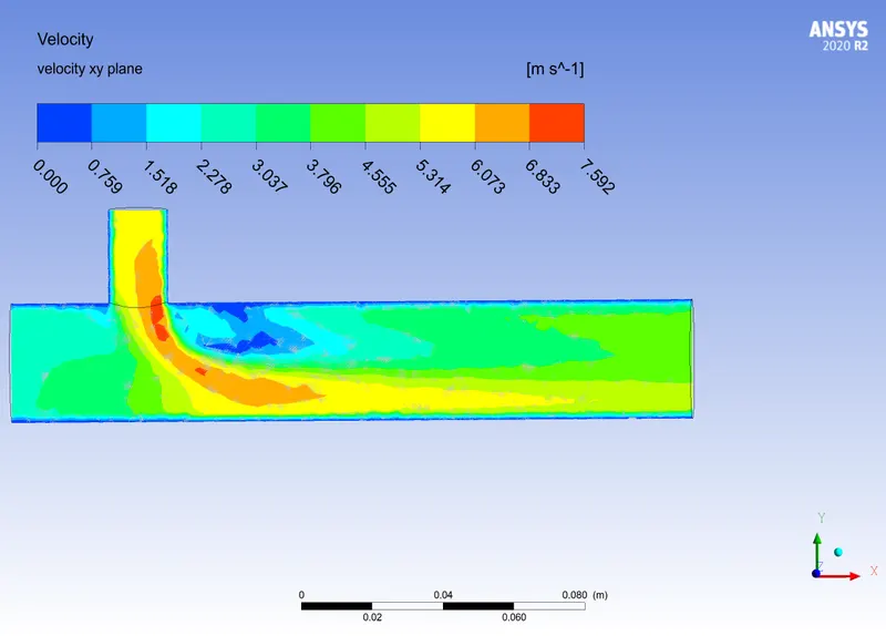
Fig 34 Contour plot for velocity in XY plane for short tee (M.R=2)

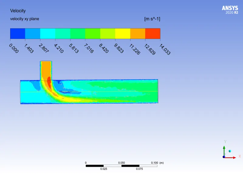
Fig 35 Contour plot for velocity in XY plane for short tee (M.R=4)

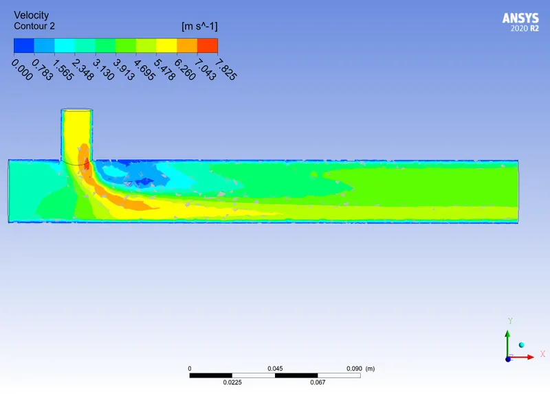
Fig 36 Contour plot for velocity in XY plane for long tee (M.R=2)

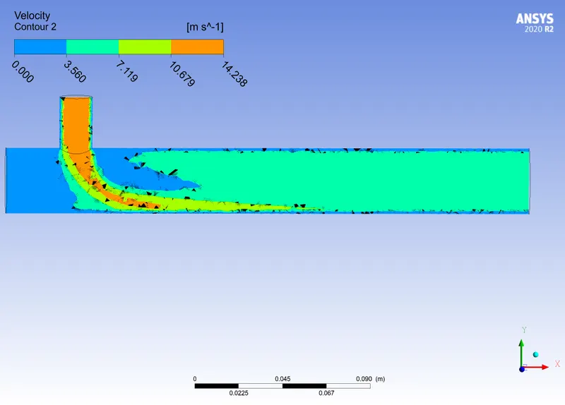
Fig 37 Contour plot for velocity in XY plane for long tee (M.R=4)

Fig 34, Fig 35, Fig 36 and Fig 37 shows the velocity profile in XY plane for all the four cases respectively. It is found that for short tee (M.R = 2) , average outlet velocity is 4.49 m/sec; for short tee (M.R = 4), average outlet velocity is 6.01 m/sec ; for long tee (M.R = 2) , average outlet velocity is 4.49 m/sec and for long tee (M.R = 4), average outlet velocity is 6 m/sec.

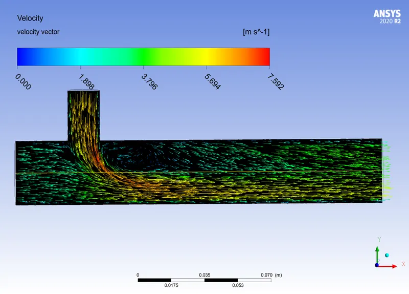
Fig 38 Vector plot for velocity vector in XY plane for short tee (M.R=2)

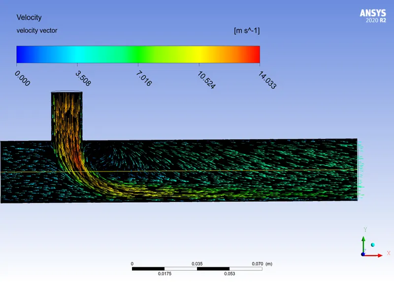
Fig 39 Vector plot for velocity vector in XY plane for short tee (M.R=4)

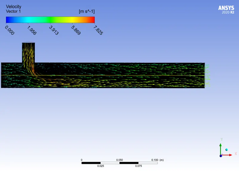
Fig 40 Vector plot for velocity vector in XY plane for long tee (M.R=2)

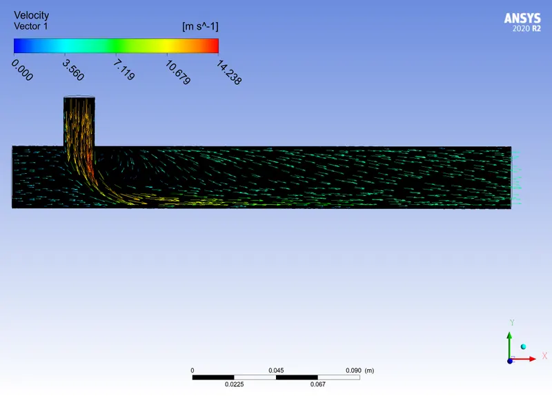
Fig 41 Vector plot for velocity vector in XY plane for long tee (M.R=4)

Fig 34, Fig 35, Fig 36 and Fig 37 shows the velocity vector profile in XY plane for all the four cases respectively. In all the four cases we can observe flow separation happening where small whirling of velocity vector is observed at the point after the intial mixing of hot and cold air takes place.

(iv) Report plots of Average outlet temperature at outlet and standard deviation of outlet temperature

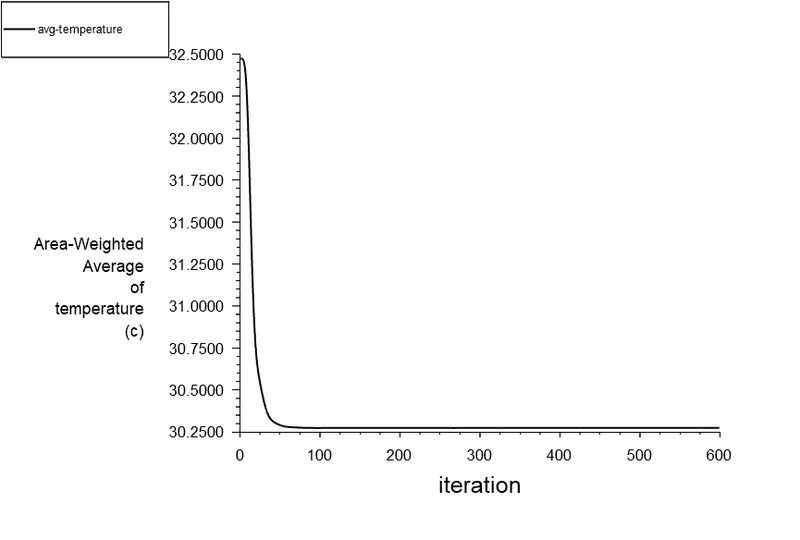
Fig 42 Area averaged outlet temperature for short tee (M.R = 2)

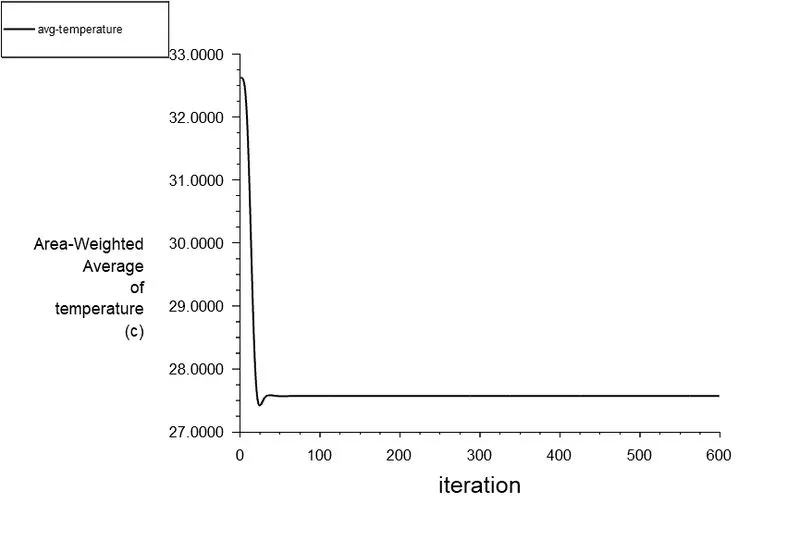
Fig 43 Area averaged outlet temperature for short tee (M.R = 4)

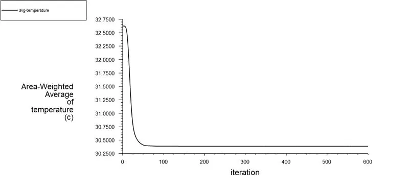
Fig 44 Area averaged outlet temperature for long tee (M.R = 2)

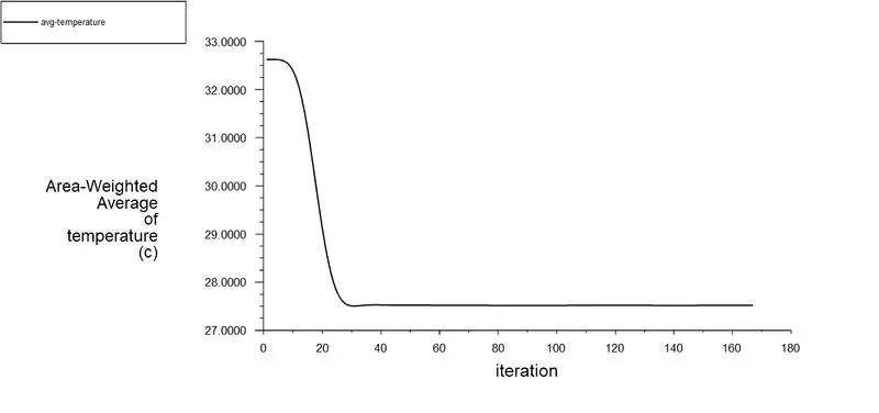
Fig 45 Area averaged outlet temperature for long tee (M.R = 4)

Fig 42, Fig 43, Fig 44 and Fig 45 shows the area averaged outlet temperature for all the four cases respectively. It is found that area averaged outlet temperature is 30.27⁰C for short tee (M.R = 2); area averaged outlet temperature is 27.56 ⁰C for short tee (M.R = 4); area averaged outlet temperature is 30.38⁰C for long tee (M.R = 2); area averaged outlet temperature is 27.51⁰C for long tee (M.R = 4).

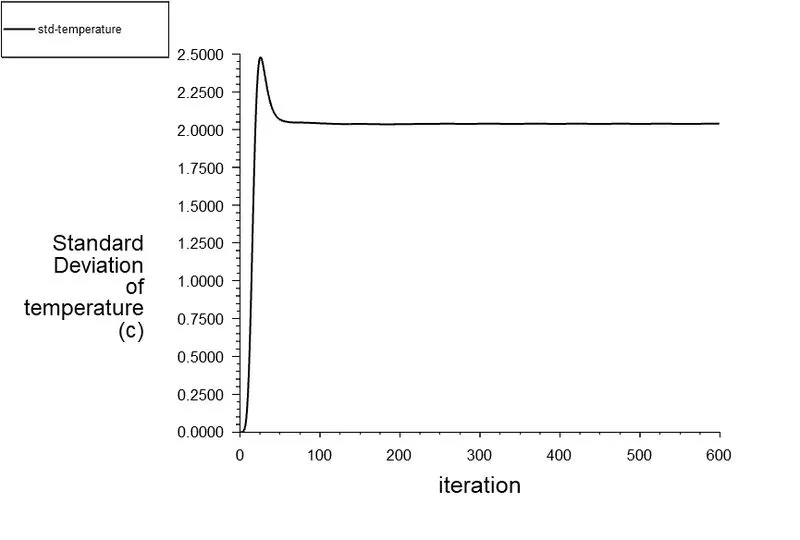
Fig 46 standard deviation of outlet temperature for short tee (M.R = 2)

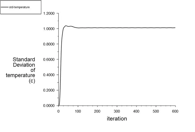
Fig 47 standard deviation of outlet temperature for short tee (M.R = 4)

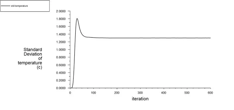
Fig 48 standard deviation of outlet temperature for long tee (M.R = 2)

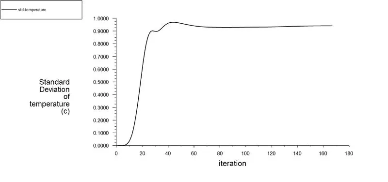
Fig 49 standard deviation of outlet temperature for long tee (M.R = 4)

Fig 46, Fig 47, Fig 48 and Fig 49 shows the standard deviation of outlet temperature for all the four cases respectively. It is found that standard deviation of temperature is 2.08⁰C for short tee (M.R = 2); standard deviation of temperature is 1⁰C for short tee (M.R = 4); the standard deviation of temperature is 1.3⁰C for long tee (M.R = 2); standard deviation of temperature is 0.94⁰C for long tee (M.R = 4). Lower the standard deviation of temperature better will be the mixing effectiveness. It is observed longer tee has higher mixing effectiveness than shorter tee for same momentum ratios.

v) Chart of temperature and velocity variation along the pipe length

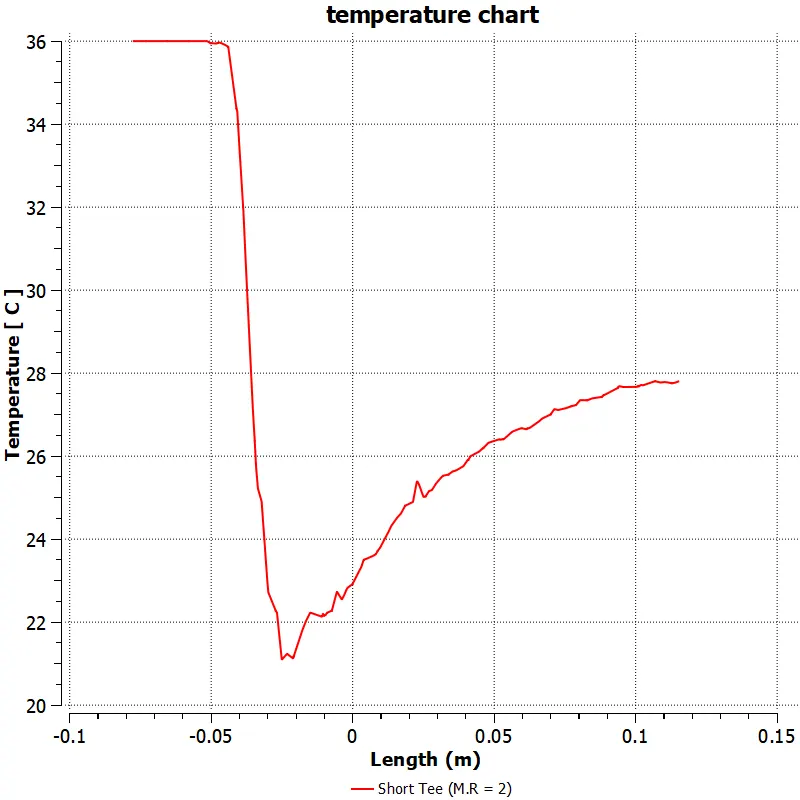
Fig 50 Temperature variation with length for short tee (M.R = 2)

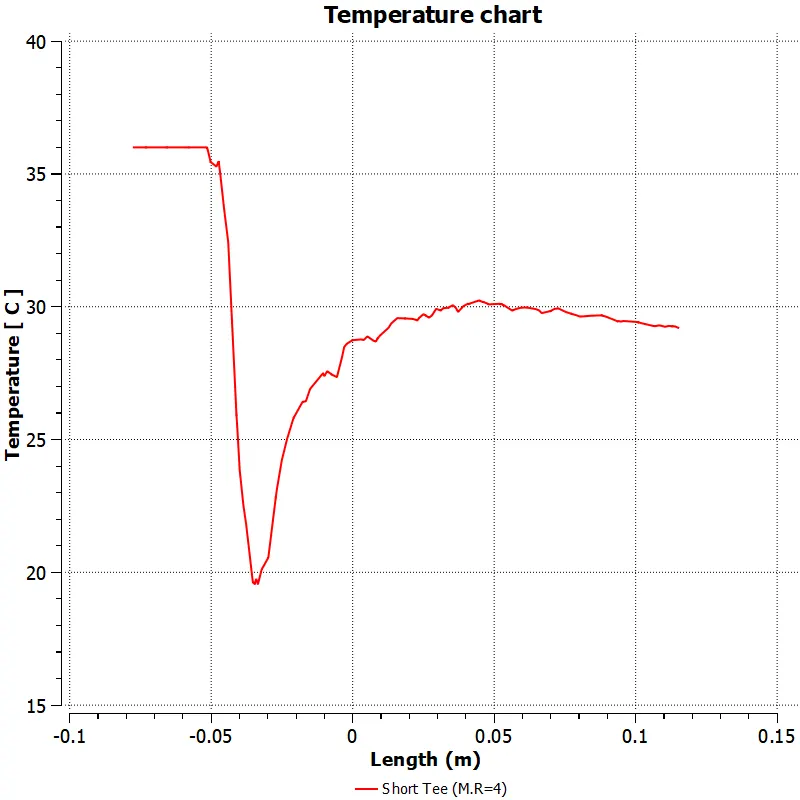
Fig 51 Temperature variation with length for short tee (M.R = 4)

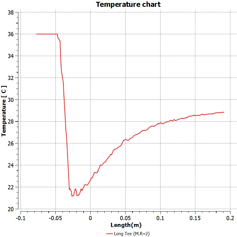
Fig 52 Temperature variation with length for long tee (M.R = 2)

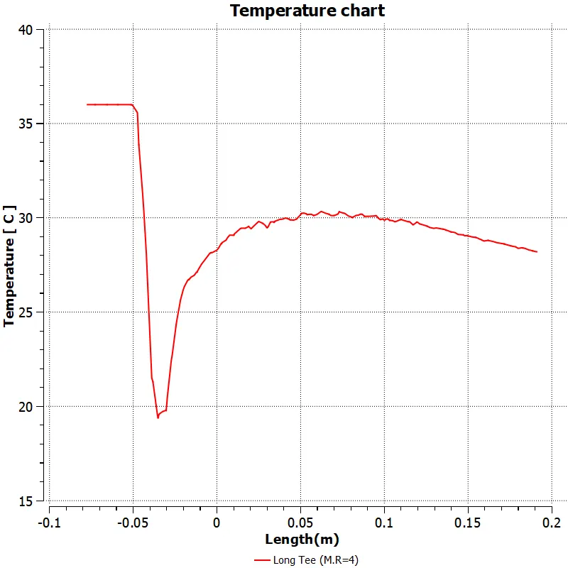
Fig 53 Temperature variation with length for long tee (M.R = 4)

A new line has been cut first in post processor and temperature variation has been calculated along the line. Fig 50, Fig 51, Fig 52 and Fig 53 shows the temperature variation along the length of the pipe in X direction. It is observed sudden drop in temperature where cold fluid is coming from the inlet and then temperature rises slowly and reaches to the steady state in all the cases.

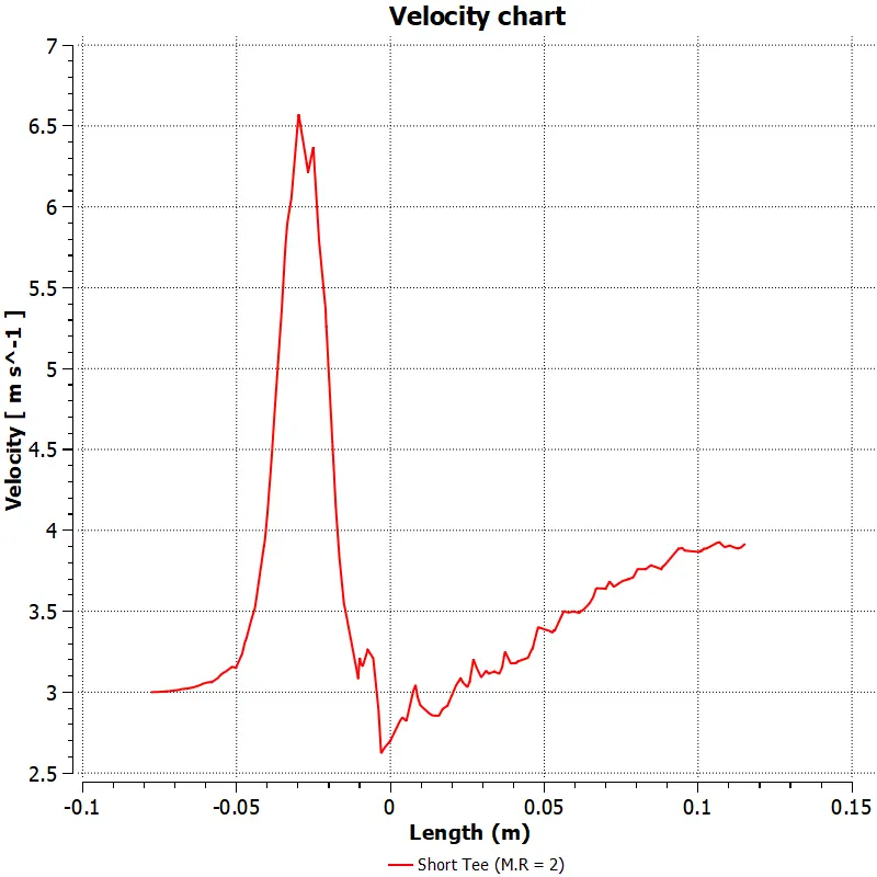
Fig 53 Velocity variation with length for short tee (M.R = 2)

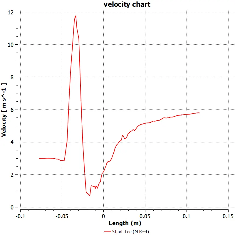
Fig 54 Velocity variation with length for short tee (M.R = 4)

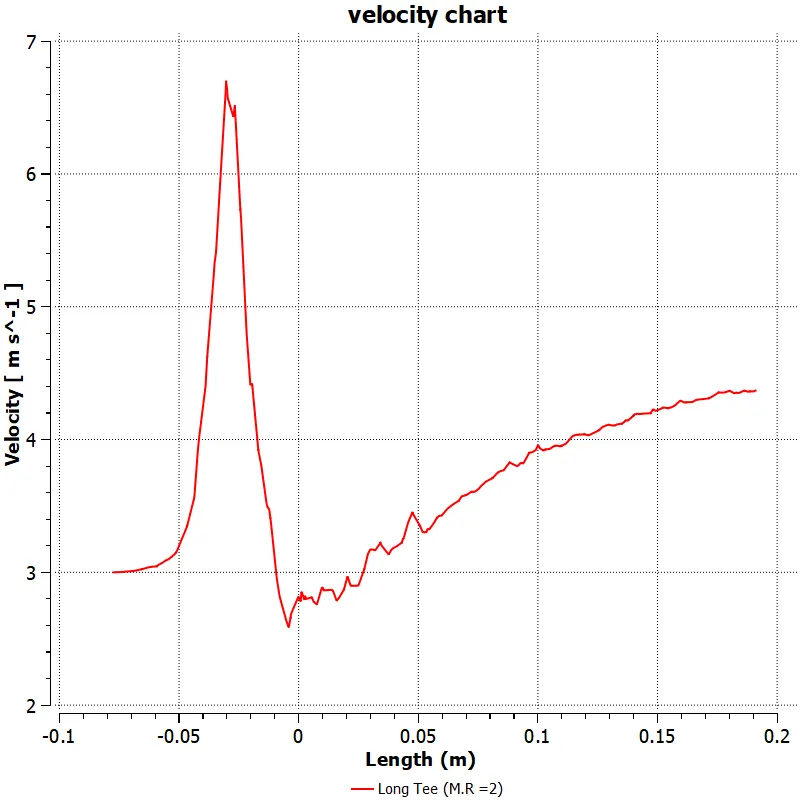
Fig 55 Velocity variation with length for long tee (M.R = 2)

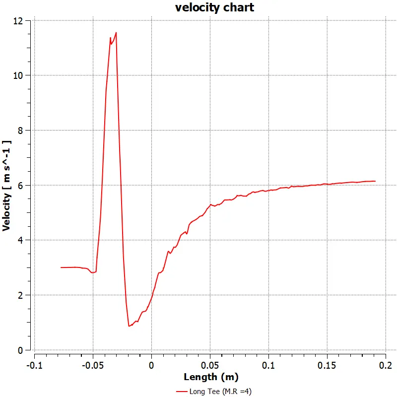
Fig 56 Velocity variation with length for long tee (M.R = 4)

Fig 53, Fig 54, Fig 55 and Fig 56 shows the velocity variation along the length of the pipe in X direction. It is observed sudden sharp rise in velocity where cold fluid is coming from the inlet and then velocity drops and then rises slowly and reaches steady state in all the cases.

Conclusions

Table 1: Variation of parameters for short and long tee for two momentum ratios

Types of Tee	Momentum ratio (M.R)	No. of elements	Avg Outlet Temperature (0C)	Avg outlet velocity (m/sec)	Std. deviation
Short Tee	2	39879	30.27	4.49	2.08
Short Tee	4	39879	27.56	6.01	1
Long Tee	2	56504	30.38	4.49	1.3
Long Tee	4	56504	27.51	6	0.94

• It is found that the length of tee doesnt have much effect on the average outlet temperature. i.e. For the same Momentum ratio, the average outlet temperature is almost same for both short tee and long tee.
• It is found that the length of tee doesnt have much effect on the average outlet velocity i.e. For the same momentum ratio, the average outlet velocity is almost same for both short tee and long tee.
• It is found that the momentum ratio has high effect on the performance of the mixing tee. i.e. When momentum ratio is increased we can observe noticable decrease in the outlet average temperature and increase in the outlet average velocity.
• It is found that the mixing effectiveness will be more when the standard deviation value is low, because then the temperature distribution is more uniform and effective mixing takes place. It is found that the mixing effectiveness of longer tee is more than the mixing effectiveness of shorter tee for the same flow conditions. It is observed that for the same tee, increasing the momentum ratio will increase the mixing effectiveness.