Week 6 - CHT Analysis on a Graphics card

Aim: To perform the steady state conjugate heat transfer on a model of graphics card for coarse and fine mesh by carying the velocity and obtain the processor temperature and surface heat transfer coefficient of the processor.

Introduction: The processor is the main part of the computer or laptop which performs many computations. Proceesor is termed as the brain of any electronic systems that incorporate into laptops, computers, smartphones and embedded systems. Although size of the processor is less, it produces more heat. Therefore, it is necessary to cool the processor to function properly. In our project, we consider an aluminium fin is attached to the silicon processor. Air is drawn towards the fin with the help of fan which is run by the battery. The speed of the air is also important, where larger the velocity the greater will be the convective heat dissipation rate from the fin. Here we are considering the conjugate heat transfer, where both conduction and convection heat transfer occurs.

Theory: In our project, the conduction heat transfer occurs throughout the wall of processor, fins while convection heat transfer takes place through the fluid (air) passing through the fin. So while designing it is necessary to make sure that both the heat transfer modes occur fast. To ensure that the conduction takes place fast we have to use higher thermal conductivity material. For processors we use silicon. Silicon is having good electrical and thermal properties. Electrical property is also important because it has to allow current to pass through the circuits faster to perform the computations. The thermal conductivity is also reasonably high for silicon, it is about 153 W/mK. For fins we use aluminium material. Its thermal conductivity is also high, it is about 203 W/mK. To increase the convection heat transfer, we can use either higher heat transfer coefficient, or higher surface area or higher temperature difference. To increase the heat transfer coefficient , we can use forced convection with the help of fan, blower or pump rather than natural convection. Also if we use liquids instead of gases, we can increase the heat transfer coefficient. In certain applications where we have to dissipate larger amount of heat from the processor we have to use liquid as the convective medium. Other way to increase the heat transfer rate was by increasing the surface area. Therefore in our fin section, we have used 15 rectangular fins which will increase the surface area, hence the convection heat transfer rate. Other way to increase the convection heat transfer is by increasing the temperature difference between the fluid and the fin surface. There are other types of cooling systems also available for processor like heat pipes, which is a passive cooling device; which means there is no need of power to run a fan; where we will utilize the circulation of a fluid, which changes to vapour on account of heat transfer from processor. Then the vapour will be moved further where they will condense , then the condensate will move through the wick structure. One advantage of this system is high heat transfer coefficient because of the phase changing occurs. In future, there is also some alternatives to silicon material in the semi conductor industry.

Solving and modelling approach:

The model is imported into the Ansys Spaceclaim, and we will remove any unwanted edges if present in the CAD cleanup. Then we will do the meshing. First we will try with the coarse mesh. So the coarse meshing is done with the base element size of 2 mm. Since processor and fin are the most important element in the computational domain so the edge sizing operation is performed on both. Since there are 15 fins, so while selecting edges of all fins, we will get 60 edges. Then edge sizing operation done, with the number of divisons as 3. Then the edge sizing operation on processor is done, with the number of divisons as 15. Then in final we will get the total number of elements as 1006163. Similarly for fine mesh we will do meshing, with the base element size of 1.5mm.Then the number of divisons given as 5 for the edge sizing operation on the fins, while for the edge sizing operation on the processor we give the number of divisons as 25. Then in final mesh we will get the total number of elements as 1595645. We will also give the named selections as inlet, outlet, enclosure, processor, fin and pcb.

Now we will do the processing in Ansys Fluent Solver. We will first enable the energy equation as we are dealing with the heat transfer. Then we will enable the k omega SST turbulence model , because we are dealing with the near wall treatment. Then we have to add silicon, polystyrene material whose properties are taken from the literature. The thermal conductivity, specific heat capacity and density of silicon are 153 W/mK , 703 J/kgK and 2330 kg/m3 respectively, while the thermal conductivity,specific heat capacity and density of polystyrene are 0.027 W/mK , 1210 J/kgK and 55 kg/m3 respectively. Then in the cell zone conditions we have to change the cell zone type as solid for processor, fin and pcb board. Then we have to give the heat source term in the processor. We suppose 2 W of heat is dissipated from the processor. Therefore we will get 31250000 W/m3 heat is dissipated (2/(8*8*1) W/mm3. Then we will give the boundary conditions. For inlet we give velocity inlet with velocity as 3m/sec. Then we will give the pressure outlet. Now we will do hybrid intialization and then we will run the calculation for 200 iterations.

Then we will obtain the report plot of the processor temperature and the processor heat transfer coefficient. In results we will obtain temperature, velocity and velocity vector for the ZX plane. Now we will run the simulation for velocity of 5 m/sec and obtain the results as above. Now we will do the analysis of finer mesh of the model compared to the previous mesh. The details of the finer mesh has been given above. Here also we will obtain the same results of processor temperature , processor heat transfer coefficient and the temperature, velocity of the air flow. The results are obtained for the velocity of 3 m/sec and 5 m/sec. We have noticed smaller processor temperature and higher processor heat transfer coefficient in velocity of 5 m/sec compared to 3 m/sec for both coarse mesh and fine mesh.

Preprocessing and solver settings:

(i) Geometry creation

The model is already created beforehand and it is imported to the Ansys Spaceclaim. The sharing topology option will be enabled so that the information will be shared across the interface and also ensure nodes of the mesh will intersect correctly at the interface.

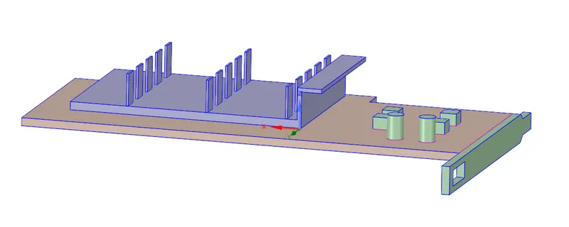
Fig 1 : Geometry of the model without enclosure

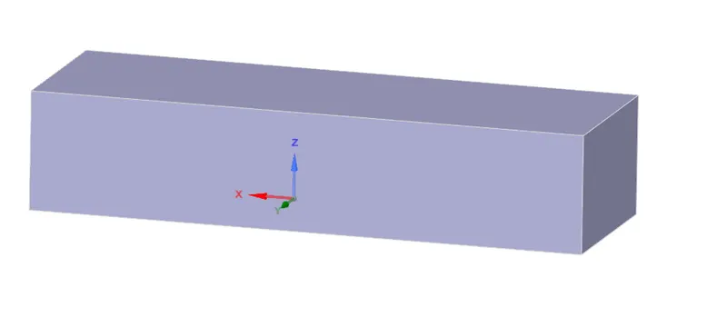
Fig 2 : Geometry of the model with enclosure

Fig 1 shows the geometry of the model without enclosure while Fig 2 shows the geometry of the model with enclosure. The enclosure is the air domain.

(ii) Meshing.

For coarse meshing, the base element size is 2 mm while the number of divisons while performing edge sizing operation on the fins and the processor were selected as 3 and 15 respectively. The total number of elements created are 1006163.

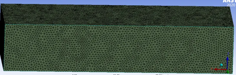
Fig 3 Meshing of the model ( coarse mesh)

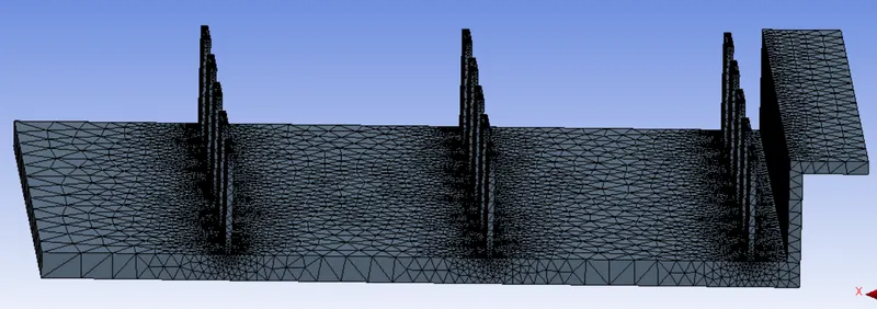
Fig 4 Meshing of the fins ( coarse mesh)

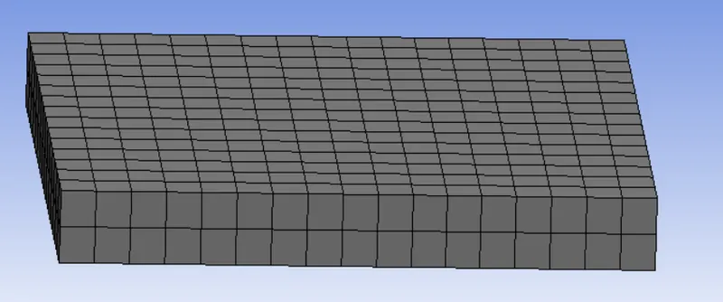
Fig 5 Meshing of the processor ( coarse mesh)

Fig 3 shows the meshing of the model while Fig 4 and Fig 5 shows the meshing of the fins and the processor respectively which is obtained by hiding the enclosure.

For fine meshing, the base element size is 1.5 mm while the number of divisons while performing edge sizing operation on the fins and the processor were selected as 5 and 25 respectively. The total number of elements created are 1595645.

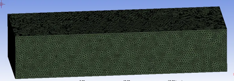
Fig 6 Meshing of the model ( fine mesh)

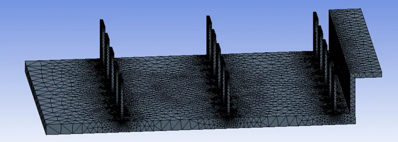
Fig 7 Meshing of the fins ( fine mesh)

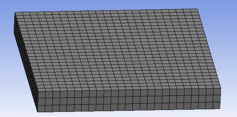
Fig 8 Meshing of the processor ( fine mesh)

Fig 6 shows the meshing of the model while Fig 7 and Fig 8 shows the meshing of the fins and the processor respectively which is obtained by hiding the enclosure.

(iii) Processing using Ansys Fluent solver

First we will enable the steady state solver with pressure based. Then we will enable the energy equation and the k omega SST turbulence model is also selected.

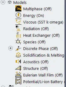
Fig 9 Model selection

Now we will add materials. Since silicon and polystyrene material is not available in the database we have to add it manually.

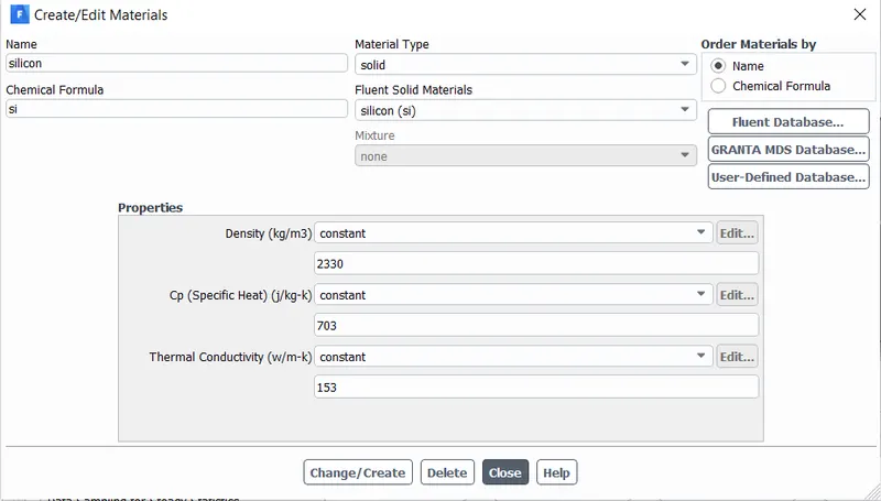
Fig 10 Silicon material selection

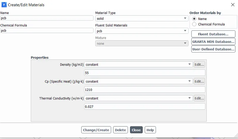
Fig 11 polystyrene material selection as pcb material

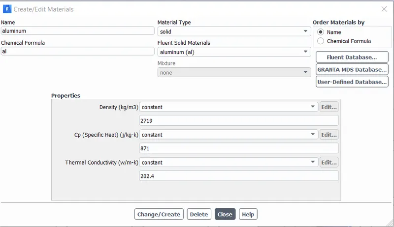
Fig 12 aluminium material selection

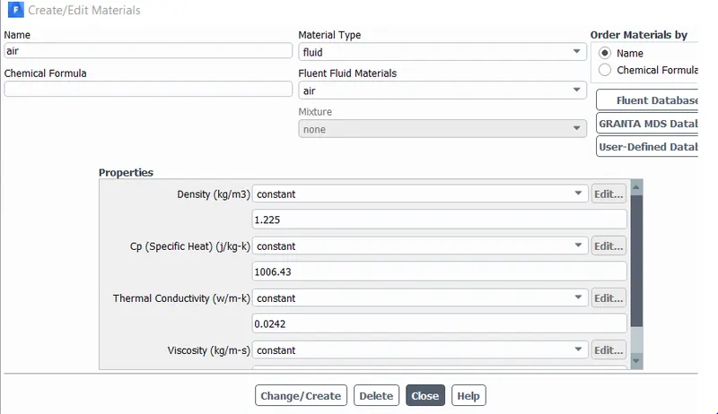
Fig 13 aluminium material selection

Now we will check the cell zone conditions and change the cell zone of processor, fin and pcb to solid from fluid. Then we will give the heat source term in the processor.

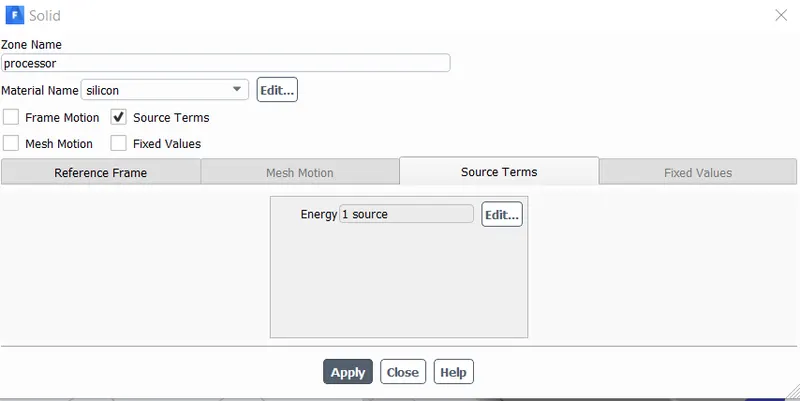
Fig 14 Enabling the source term in the processor

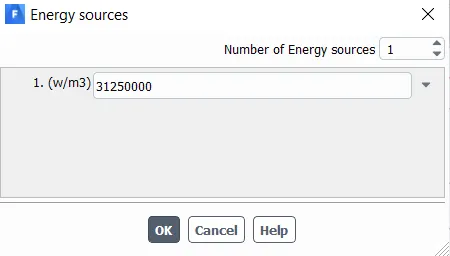
Fig 15 Specifying the source term in the processor

Now we will give the boundary conditions. We will give the velocity inlet condition and the pressure outlet condition. For the first case we will give the inlet velocity of 3 m/sec and the second case we we will give velocity of 5 m/sec

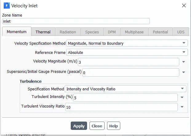
Fig 16 Specifying the inlet velocity of 3m/sec

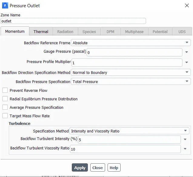
Fig 17 Specifying pressure outlet

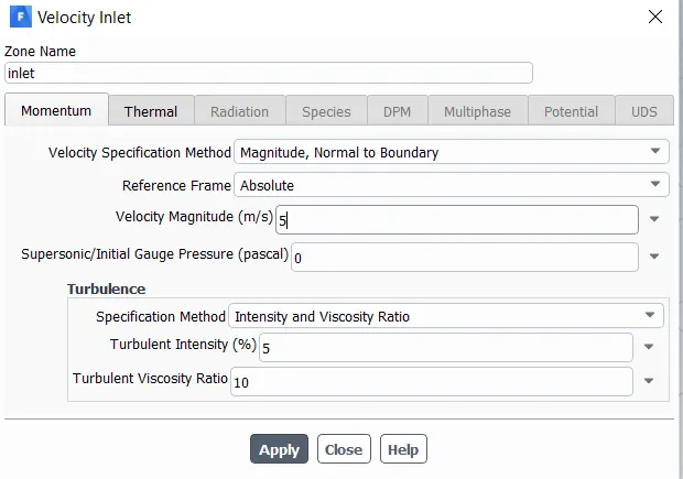
Fig 16 Specifying the inlet velocity of 5m/sec

Now we will go to the solution methods. We will use the default settings.

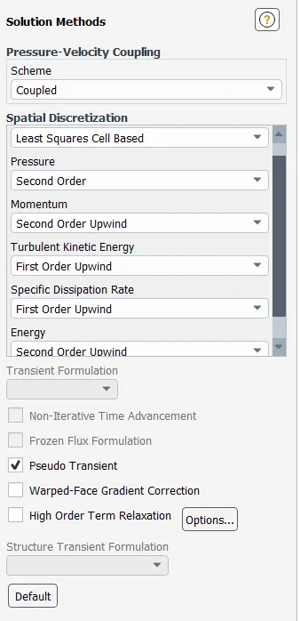
Fig 17 Specifying the solution methods

We will now create the new report definitions. First we will create area average of static temperature of the procesor. Next is the area average of the surface heat transfer coefficient of the processor.

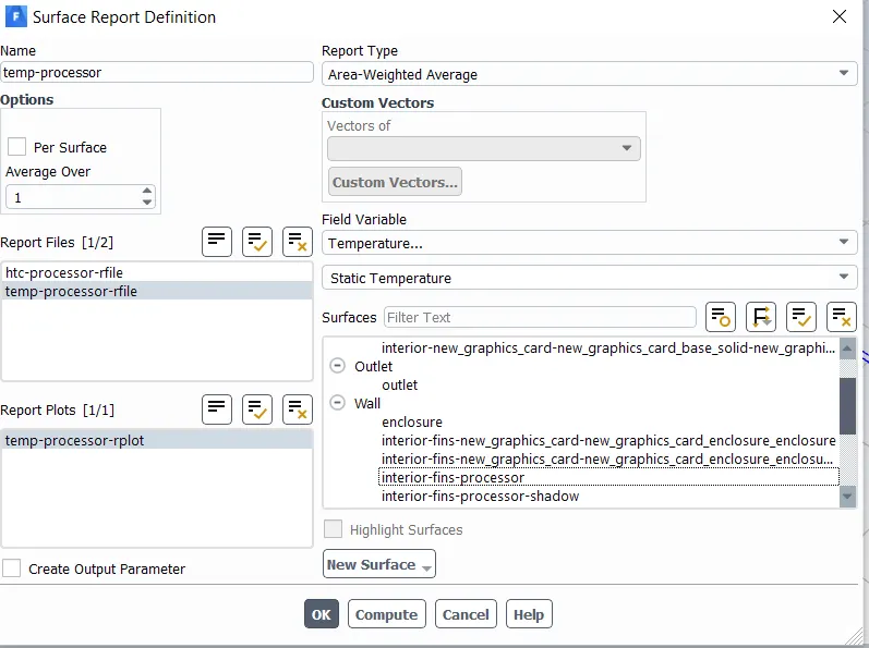
Fig 18 Surface report creation of static temperature of processor

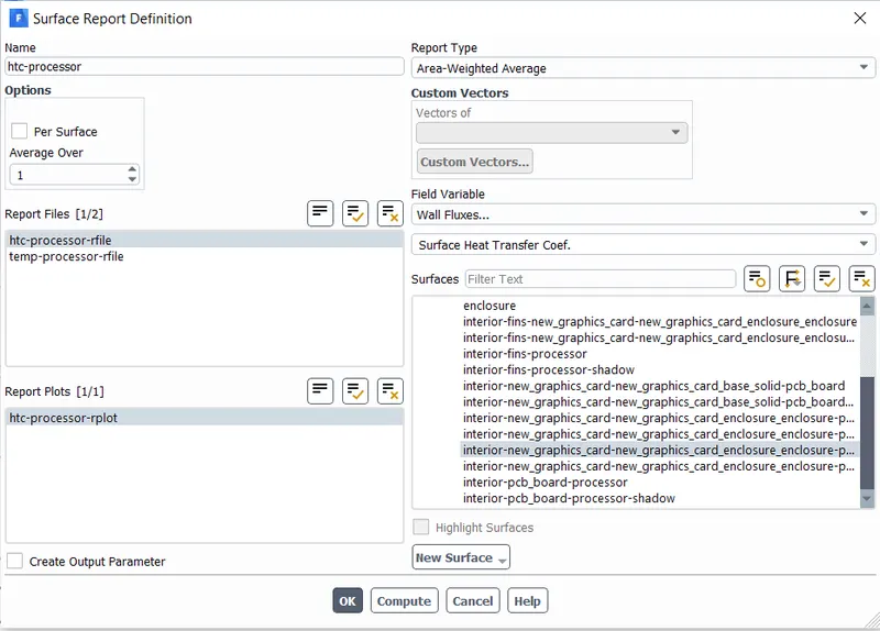
Fig 19 Surface report creation of surface heat transfer coefficient of processor

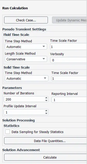
Fig 20 Specifying the iterations in calculation

Now we will run the calculation for 200 iterations until we will get convergence.

Results:

(i) Residual plots

a For Coarse Mesh for inlet velocity of 3 m/sec

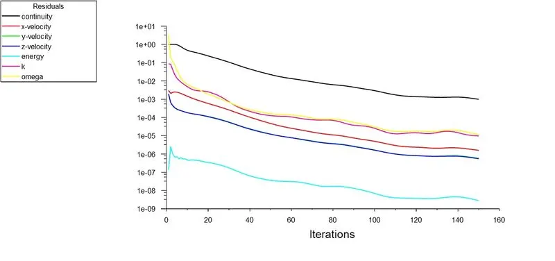
Fig 21 Residual plot for coarse mesh for inlet velocity of 3m/sec

b For Coarse Mesh for inlet velocity of 5 m/sec

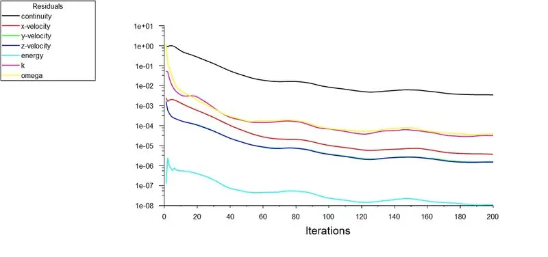
Fig 22 Residual plot for coarse mesh for inlet velocity of 5m/sec

c For fine Mesh for inlet velocity of 3 m/sec

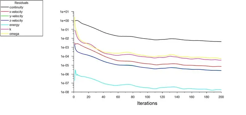
Fig 23 Residual plot for coarse mesh for inlet velocity of 3m/sec

d For fine Mesh for inlet velocity of 5 m/sec

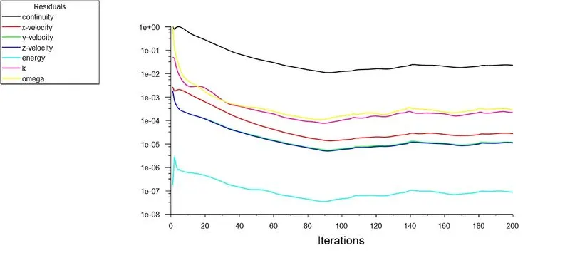
Fig 24 Residual plot for coarse mesh for inlet velocity of 5m/sec

We have run the calculation for 200 iterations in all the four cases and have attained convergence by that time.

(ii) Processor temperature

a For Coarse Mesh for inlet velocity of 3 m/sec

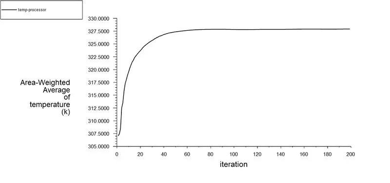
Fig 25 Processor temperature for coarse mesh for inlet velocity of 3 m/sec

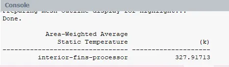
Fig 26 Console report of processor temperature

Fig 25 shows the processor temperature for coarse mesh for inlet velocity of 3 m/sec while Fig 26 shows its console report and the avg. processor temperature is 327.91K

b For Coarse Mesh for inlet velocity of 5 m/sec

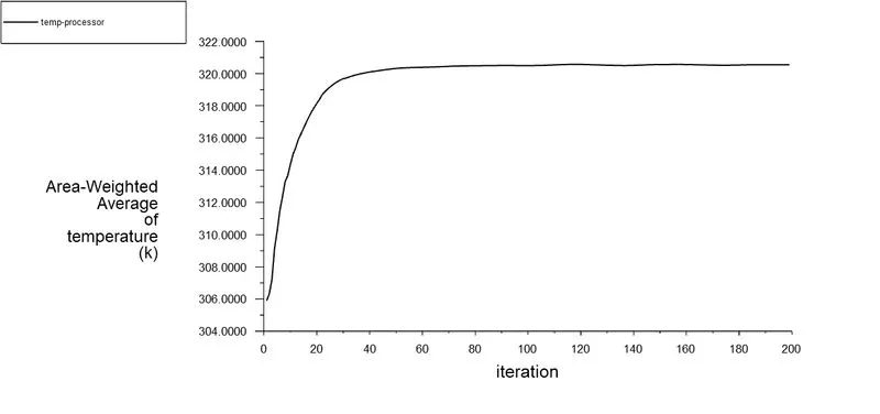
Fig 27 Processor temperature for coarse mesh for inlet velocity of 3 m/sec

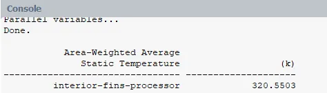
Fig 28 Console report of processor temperature

Fig 27 shows the processor temperature for coarse mesh for inlet velocity of 5 m/sec while Fig 28 shows its console report and the avg. processor temperature is 320.55K

c For Fine Mesh for inlet velocity of 3 m/sec

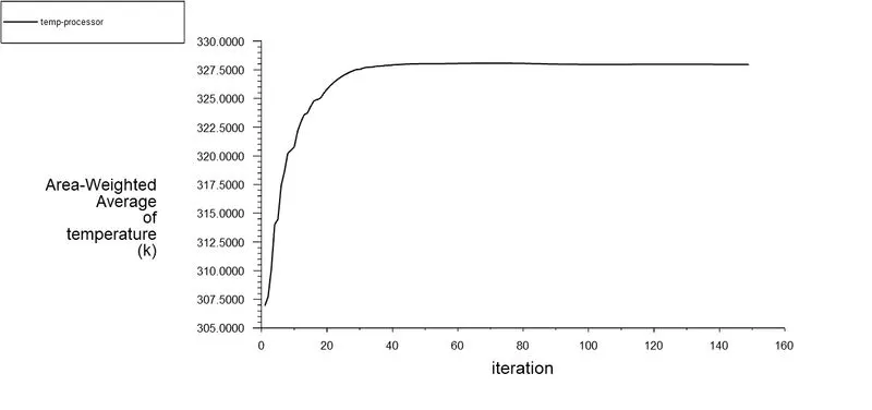
Fig 29 Processor temperature for fine mesh for inlet velocity of 3 m/sec

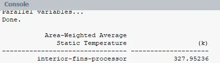
Fig 30 Console report of processor temperature

Fig 29 shows the processor temperature for fine mesh for inlet velocity of 3 m/sec while Fig 30 shows its console report and the avg. processor temperature is 327.95 K

c For Fine Mesh for inlet velocity of 5 m/sec

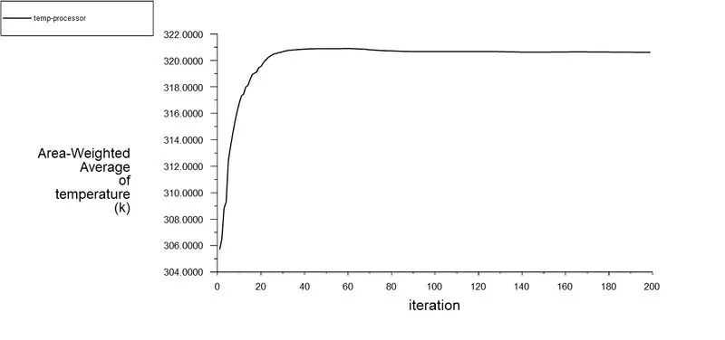
Fig 31 Processor temperature for fine mesh for inlet velocity of 5 m/sec

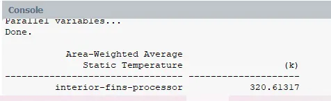
Fig 32 Console report of processor temperature

Fig 31 shows the processor temperature for fine mesh for inlet velocity of 5 m/sec while Fig 32 shows its console report and the avg. processor temperature is 320.61 K

(iii) Surface heat transfer coefficient of processor

a For Coarse Mesh for inlet velocity of 3 m/sec

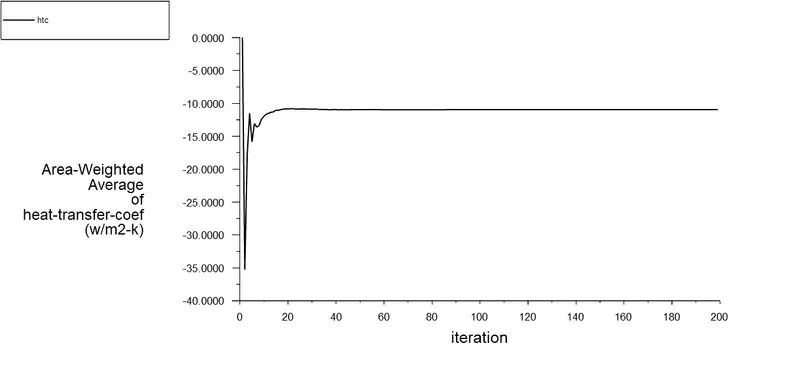
Fig 33 Processor surface heat transfer coefficient for coarse mesh for inlet velocity of 3 m/sec

Fig 34 Console report of heat transfer coefficient of processor

Fig 33 shows the processor surface heat transfer coefficient for coarse mesh for inlet velocity of 3 m/sec while Fig 34 shows the console report value and it is - 10.94 W/m2K. Negative sign indicates the heat flows away from the fin surface.

b For Coarse Mesh for inlet velocity of 5 m/sec

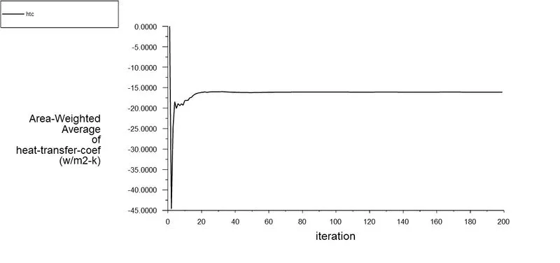
Fig 35 Processor surface heat transfer coefficient for coarse mesh for inlet velocity of 5 m/sec

Fig 36 Console report of heat transfer coefficient of processor

Fig 35 shows the processor surface heat transfer coefficient for coarse mesh for inlet velocity of 5 m/sec while Fig 36 shows the console report value and it is - 16.09 W/m2K.

c For fine Mesh for inlet velocity of 3 m/sec

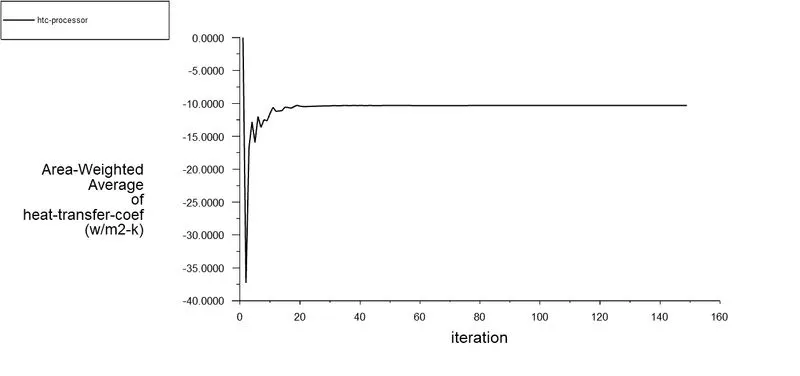
Fig 37 Processor surface heat transfer coefficient for fine mesh for inlet velocity of 3 m/sec

Fig 38 Console report of heat transfer coefficient of processor

Fig 37 shows the processor surface heat transfer coefficient for fine mesh for inlet velocity of 3 m/sec while Fig 38 shows the console report value and it is - 10.31 W/m2K.

d For fine Mesh for inlet velocity of 5 m/sec

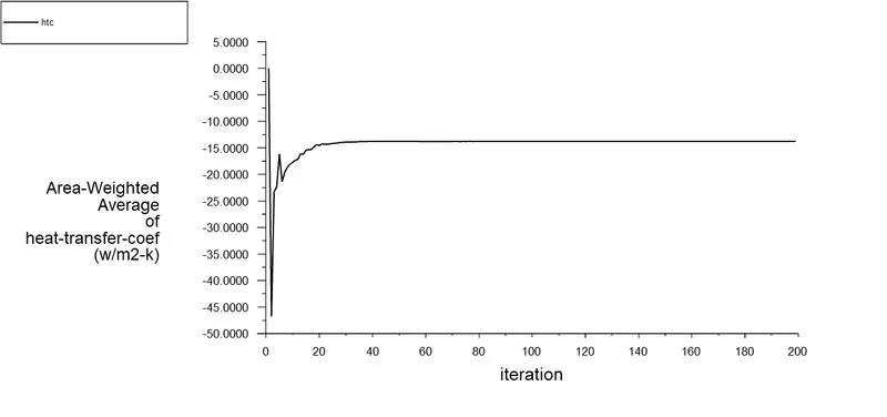
Fig 39 Processor surface heat transfer coefficient for fine mesh for inlet velocity of 5 m/sec

Fig 40 Console report of heat transfer coefficient of processor

Fig 39 shows the processor surface heat transfer coefficient for fine mesh for inlet velocity of 5m/sec while Fig 40 shows the console report value and it is - 13.76 W/m2K.

(iv) Flow velocity

a For Coarse Mesh for inlet velocity of 3 m/sec

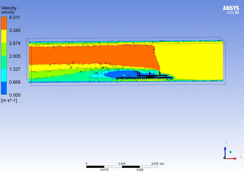
Fig 41 Velocity of air flow contour for coarse mesh for 3 m/sec

b For Coarse Mesh for inlet velocity of 5 m/sec

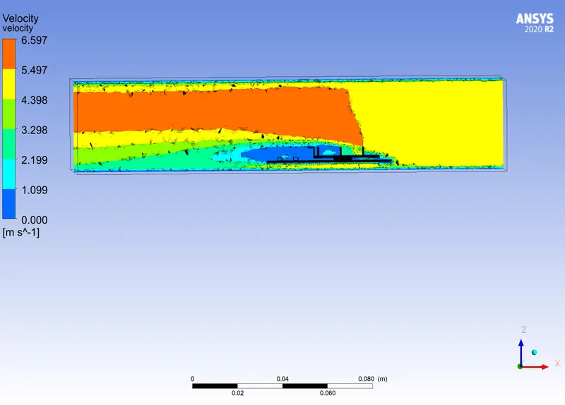
Fig 42 Velocity of air flow contour for coarse mesh for 5 m/sec

c For fine Mesh for inlet velocity of 3 m/sec

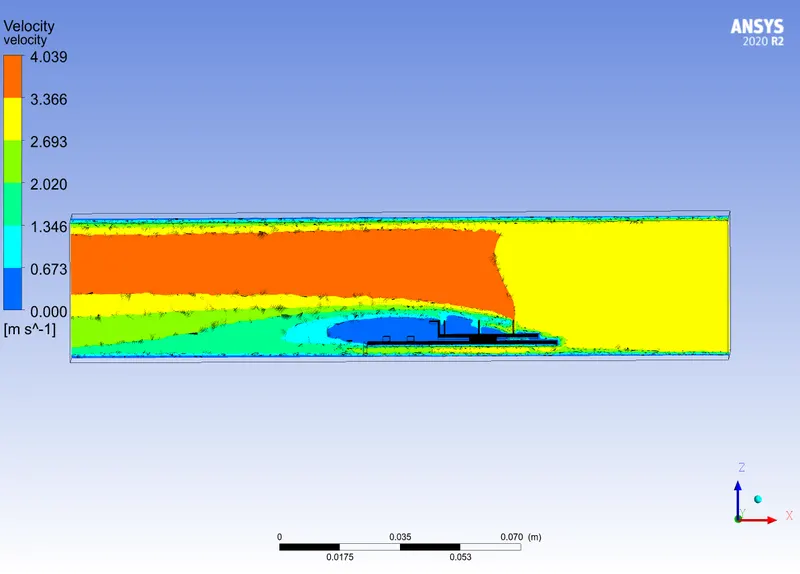
Fig 43 Velocity of air flow contour for coarse mesh for 3 m/sec

d For fine Mesh for inlet velocity of 5 m/sec

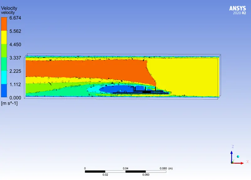
Fig 44 Velocity of air flow contour for coarse mesh for 5 m/sec

(v) 3 D Temperature contour

a For coarse Mesh for inlet velocity of 3 m/sec

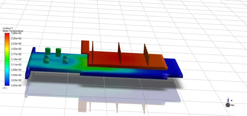
Fig 45 Temperature distribution for coarse mesh for inlet velocity of 3 m/sec

b For coarse Mesh for inlet velocity of 5 m/sec

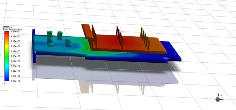
Fig 46 Temperature distribution for coarse mesh for inlet velocity of 5 m/sec

c For fine Mesh for inlet velocity of 3 m/sec

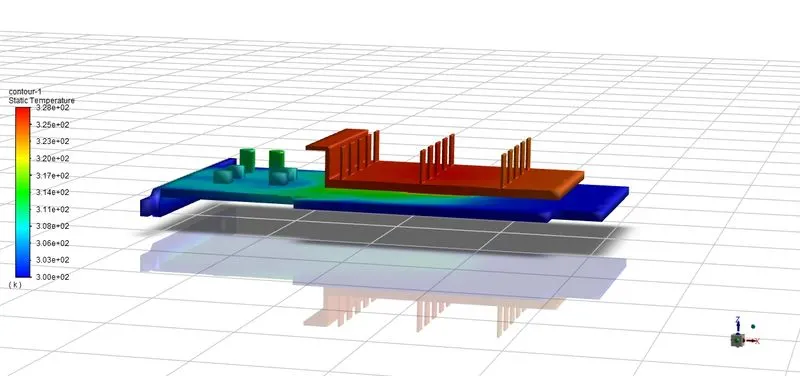
Fig 47 Temperature distribution for fine mesh for inlet velocity of 5 m/sec

d For fine Mesh for inlet velocity of 5 m/sec

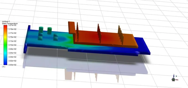
Fig 48 Temperature distribution for fine mesh for inlet velocity of 5 m/sec

(vi) Velocity vector plot

a For coarse Mesh for inlet velocity of 3 m/sec

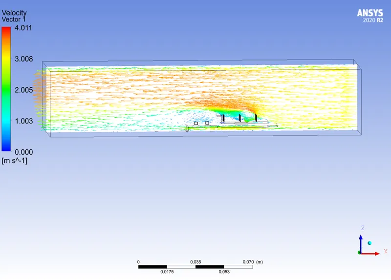
Fig 49 Velocity vector plot for coarse mesh for inlet velocity of 3m/sec

b For coarse Mesh for inlet velocity of 5 m/sec

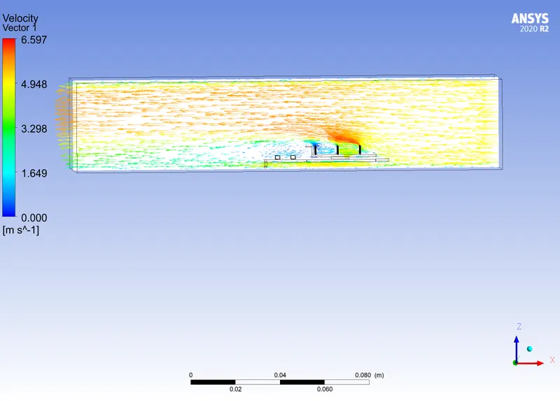
Fig 50 Velocity vector plot for coarse mesh for inlet velocity of 5m/sec

c For fine Mesh for inlet velocity of 3 m/sec

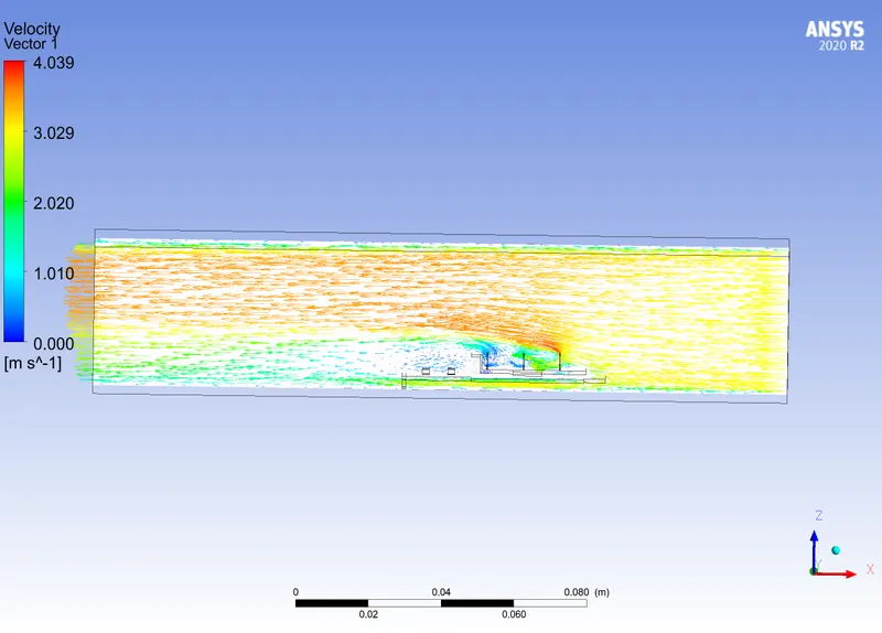
Fig 51 Velocity vector plot for fine mesh for inlet velocity of 3m/sec

d For fine Mesh for inlet velocity of 5 m/sec

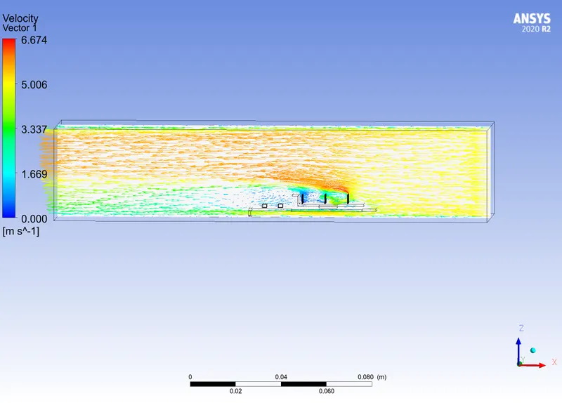
Fig 52 Velocity vector plot for fine mesh for inlet velocity of 3m/sec

Conclusions:

We have done the CHT simulation on graphics card for both coarse and fine mesh with inlet velocity of 3 m/sec and 5 m/sec. The total number of mesh elements obtained for coarse mesh is 1006163, while for fine mesh is 1595645.

S No	Mesh Type	Inlet velocity (m/sec)	Processor Avg Temperature (K)	Processor Avg heat transfer coefficient (W/m2K)
1	Coarse	3	, 327.91	10.94
2	Fine	3	327.95	10.31
3	Coarse	5	320.55	16.09
4	Fine	5	320.61	13.76

• It is observed that while comparing between coarse and fine mesh there is no significant difference seen in the average processor temperature for both inlet velocity cases of 3 m/sec and 5 m/sec.
• The heat transfer coefficient results also show less difference, but in case of 5 m/sec inlet velocity, we can observe slight deviation, with the heat transfer coefficient obtained for coarse mesh is 16.09 W/m2K while for fine mesh is 13.76 W/m2K