Week 8 - Simulating Cyclone separator with Discrete Phase Modelling

Aim: To perform analysis on cyclone separator and calculate the separation efficiency and pressure drop.

Objectives

1. Brief introduction to 4 empirical models used to calculate the cyclone separator efficiency.
2. To perform an analysis on a given cyclone separator model by varying the particle diameter from 1 μm to 5 μm and calculate the separation efficiency in each case and discuss the results.
3. To perform an analysis on a given cyclone separator model by varying the particle velocity from 1 m/sec to 5 m/sec and calculate the separation efficiency and pressure drop in each case and discuss the results.

Cyclone Separator

Cyclone separators are separation devices that use the principle of inertia to remove particulate matter from flue gases.

In a cyclone separator, dirty flue gas is fed into a chamber.

The inside of the chamber creates a spiral vortex

The lighter components of this gas which have less inertia get easily influenced by the vortex and travel upwards towards the upper outlet.

The larger components of particulate matter have more inertia and are not as easily influenced by the vortex

Since these larger particles have difficulty following the high-speed spiral motion of the gas and the vortex, the particles hit the inside walls of the container and drop down into a collection hopper. These chambers are shaped like an upside-down cone to promote the collection of these particles at the bottom of the container.

The cleaned flue gas escapes out the top of the chamber.

Uses: Air Pollution Control, Dust Collector

Empirical Models used to calculate cyclone separator efficiency

1. Iozia and Leith

Iozia and Leith logistic model is a modified version of Barth Model, which is developed based on force balance.

The model assumes that a particle carried by the vortex endures the influence of two forces: a centrifugal force, Z and a flow resistance, W.

The collection efficiency η_i of particle diameter d_pi can be calculated from

`ηi=1(1+(dpc)/(dp,i))^β`

β is an expression for slope parameter derived based on the

statistical analysis of experimental data of a cyclone with D =0.25 m given as

`β = 0.62 - 0.87 ln (dpc/100) + 5.21 ln (ab/D^2) + 1.05 〖(ln (ab/D^2))〗^2`

where d_pc is 50% cut size given by Barth.

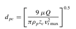
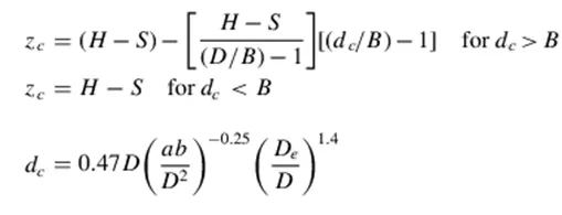
where core length, z_c , and core diameter, d_c, are given as

2. Li and Wang Model

The Li and Wang model includes particle bounce or re-entrainment and turbulent diffusion at the cyclone wall.

A two-dimensional analytical expression of particle distribution in the cyclone is obtained.

Li and Wang model was developed based on the following assumptions:

• The radial particle velocity and the radial concentration profile are not constant for uncollected particles within the cyclone.
• Boundary conditions with the consideration of turbulent diffusion coefficient and particle bounce re- entrainment on the cyclone wall are
• The tangential velocity is related to the radius of cyclone by: uRⁿ = constant.

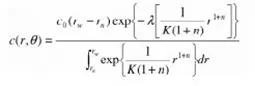
The concentration distribution in a cyclone is given as:

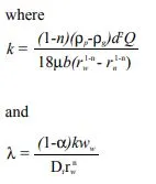
The resultant expression of the collection efficiency for particle of my size is given as

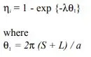
3. KOCH AND LICHT MODEL
   This Model recognizes the inherently turbulent nature of cyclones and the distribution of gas residence times within the cyclone. It describes particle motion in the entry and the collection regions with some assumptions,
   The tangential velocity of particles is equal to the tangential velocity of the gas flow i.e. 'no slip' in tangential direction between the particle and the gas.
   2. The tangential velocity is related to the radius of the cyclone by UR^n = constant
   A force balance and the equation on this particles collection yield the grade efficiency,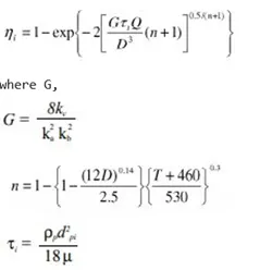
   

G is a factor related to the configuration of the cyclone, n is related to the vortex and τ is the relaxation term.

4. LAPPLE MODEL
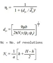
   It is a 1951 model developed by LAPPLE assuming that a particle entering a cyclone is evenly distributed along with the inlet opening. It is based on Force Balance without considering the flow resistance. In this model, the particle that travels from inlet half-width to the wall in the Cyclone is collected with 50% efficiency.
   Efficiency,
   

Pre-processing

Geometry:

Volume Extracted

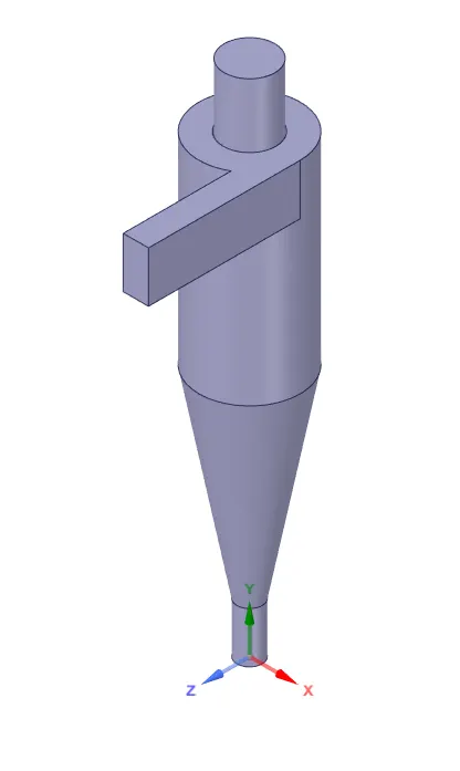
Mesh

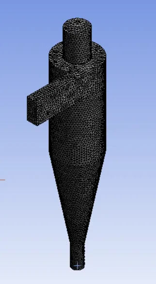
Mesh Details

Element Size: 10mm

Nodes: 22951

Elements: 112565

SOLVER SETUP

Solver: Steady State, Pressure Based

Gravity: 9.81 m/s in -Y direction

Turbulence Model: RNG K-epsilon ( Swirl Dominated Flow)

DPM Iteration Interval: 10

Max Steps: 50,000
Step Length Factor: 5

Injections
Type: Surface
Material: Anthracite

Case 1
Velocity: 3 m/s
Diameter: 1-5 micrometres

Case 2

Diameter: 5 micrometres

Velocity: 1-5 m/s

Boundary Conditions

Inlet: DPM – Reflect

Outlet 1: DPM- Escape

Outlet 2: DPM – Trap

Solution methods
Pressure Velocity Coupling Scheme: Coupled

Spacial discretization

Pressure: Second Order

Momentum: Second Order Upwind

Turbulent Kinetic Energy: Second Order Upwind
Turbulent Dissipation Rate: Second Order Upwind

Initialization: Standard

Time Scale Factor: 1

Iterations: 600

SOLUTION

Case 1

Velocity: 3 m/s

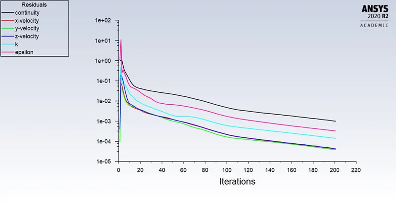
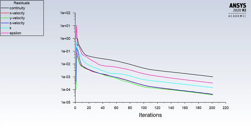
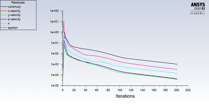
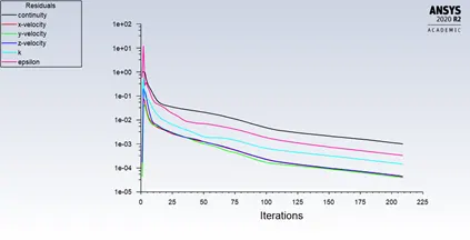
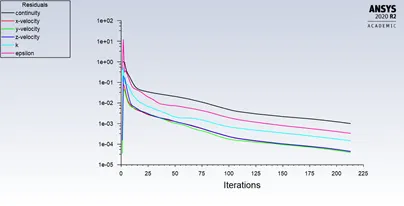
Residuals

1 micrometre	2 micrometres	3 micrometres
4 micrometres	5 micrometres

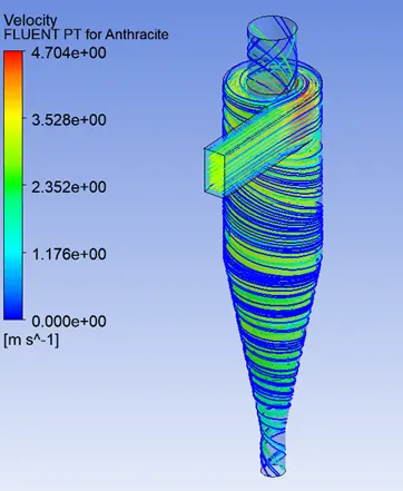
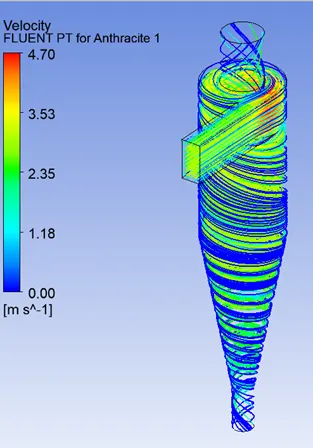
Velocity

1 micrometre	2 micrometres	3 micrometres
4 micrometres	5 micrometres

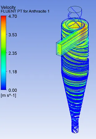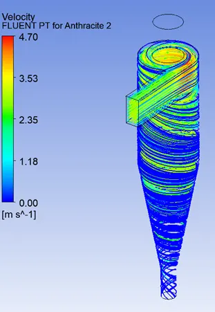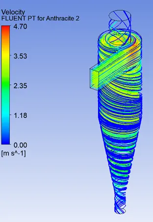
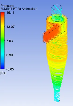
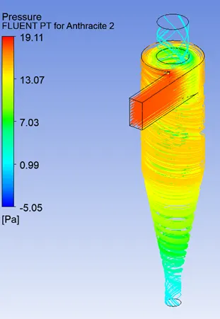
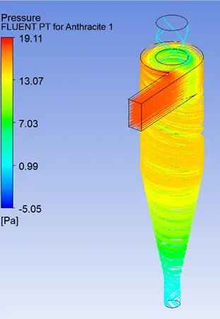
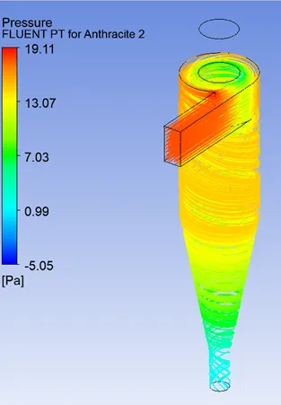
Pressure

1 micrometre	2 micrometres	3 micrometres
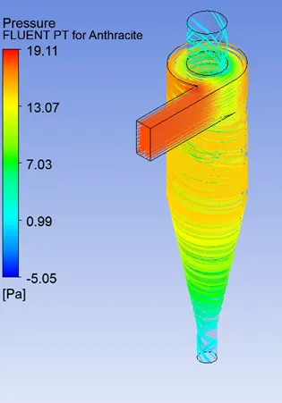4 micrometres	5 micrometres

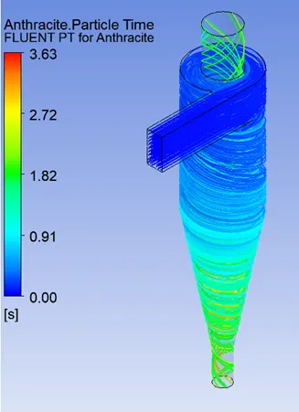
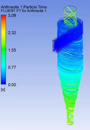
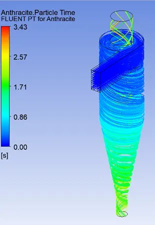
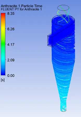
Particle Time

1 micrometre	2 micrometres	3 micrometres
4 micrometres	5 micrometres

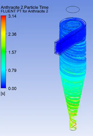Diameter	Tracked	Escaped	Trapped	Seperation efficiency
1	124	24	41	.33
2	124	22	98	.77
3	124	18	106	.85
4	124	6	117	.94
5	124	0	124	1

Case 2

Particle diameter: 5 micrometres

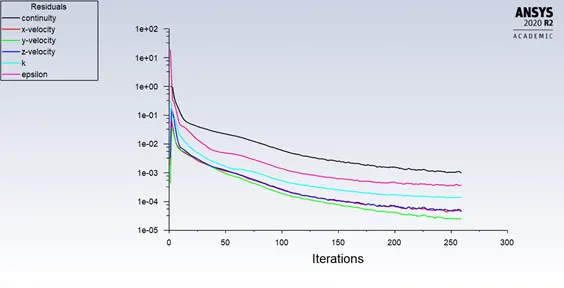
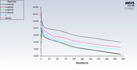
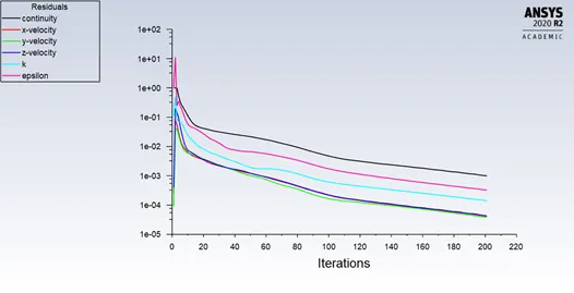
Residuals

1 m/s	2 m/s	3 m/s
4 m/s	5 m/s

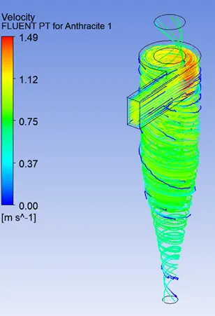
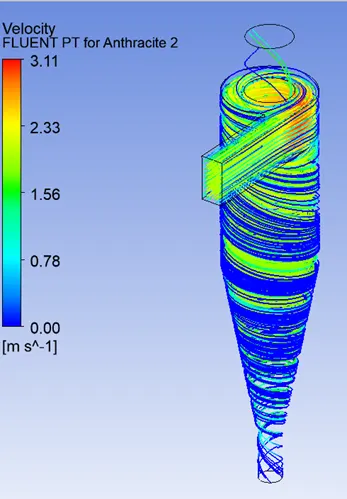
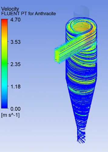
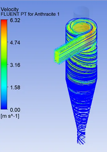
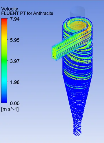
Velocity

1 m/s	2 m/s	3 m/s
4 m/s	5 m/s

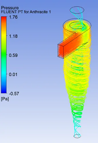
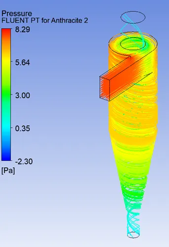
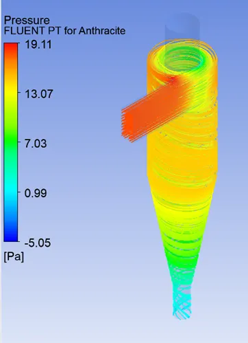
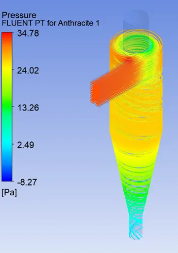
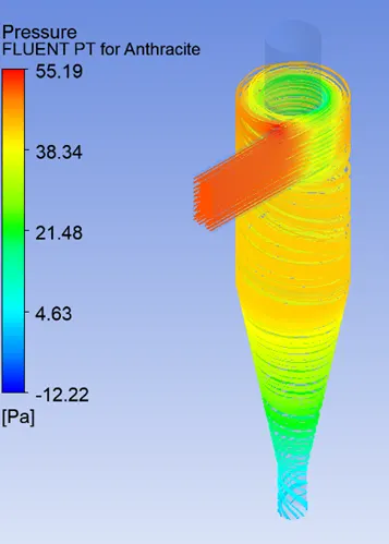
Pressure

1 m/s	2 m/s	3 m/s
4 m/s	5 m/s

z

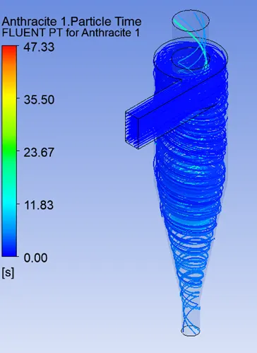
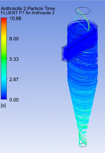
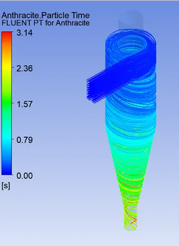
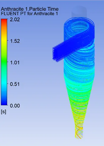
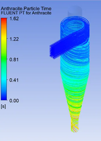
Particle Time

1 m/s	2 m/s	3 m/s
4 m/s	5 m/s

Observations

Velocity	Tracked	Escaped	Trapped	Separator efficiency	Pressure Drop
1	124	6	9	.07	2.33
2	124	4	31	.25	10.59
3	124	0	124	1	24.16
4	124	0	124	1	43.05
5	124	0	124	1	67.41

RESULTS

CASE 1

Diameter	Tracked	Escaped	Trapped	Seperation efficiency
1	124	24	41	.33
2	124	22	98	.77
3	124	18	106	.85
4	124	6	117	.94
5	124	0	124	1

CASE 2

Velocity	Tracked	Escaped	Trapped	Separator efficiency	Pressure Drop
1	124	6	9	.07	2.33
2	124	4	31	.25	10.59
3	124	0	124	1	24.16
4	124	0	124	1	43.05
5	124	0	124	1	67.41

OBSERVATIONS

The number of trapped particles increase with increase in diameter and velocity

When the velocity is kept constant, the separation efficiency increases with particle size and the pressure drop remains constant

When the particle size is kept constant, the separation efficiency and pressure drop increase with increase in velocity