Week 8 - Simulating Cyclone separator with Discrete Phase Modelling

Objective:

To conduct studies on the cyclone separator and determine the efficiency of the separation as well as the pressure drop. Conduct the study with velocities ranging from one meter per second to five meters per second and with particle sizes ranging from one micrometer to five micrometers. Compile the findings into a table, then evaluate their usefulness.

Introduction:

Vortex separation is a way to get rid of particles in a stream of air, gas, or liquid without using filters. This is called cyclonic separation. A hydrocyclone is used to remove particles from liquids, while a gas cyclone is used for gases. Solids and liquids that are mixed together can be separated with the help of rotation and gravity. You can also use the method to separate small drops of liquid from a stream of gas.
A cyclone is a cylindrical or conical container that sets up a high-speed rotating flow of air. Air flows in a spiral, starting at the top (wide end) and ending at the bottom (narrow end) of the cyclone. It then goes straight through the centre of the cyclone and out the top. Larger (denser) particles in the rotating stream have too much momentum to follow the tight curve of the stream. Instead, they hit the outside wall and fall to the bottom of the cyclone, where they can be removed. In a conical system, as the rotating flow moves toward the narrow end of the cyclone, the stream's rotational radius decreases, separating smaller and smaller particles. The cut point of a cyclone is determined by the shape and flow rate of the cyclone. This is the size of the particle that will be taken out of the stream 50% of the time. Particles bigger than the cut point will be removed more efficiently, while smaller particles will be removed less efficiently because they are harder to separate or can get pulled back in when the air vortex changes direction and moves toward the outlet.

How things work:

Under a certain amount of pressure, the product is fed into the cyclone separator at an angle. This makes a spinning movement that pushes the heavier phase out and down along the wall of the cone-shaped part. As the diameter gets smaller in the conical part, the speed goes up, which helps the separation. Last, the solids that have been concentrated are let out through the top. The vortex finder in the overflow part makes the fluid move quickly in an upward spiral in the middle of the cone-shaped housing. Through the overflow outlet, the fluid is let out.

Parameters for good cyclone operation :

• The design.
• The specific weight difference between the two product phases.
• The shape of the solids.
• The speed of the feed.
• The density of the medium.
• The counter pressure at the overflow and apex.

The following are some of the empirical models that are used in the calculation of the cyclone separator's efficiency:

1) IOZIA AND LEITH MODEL :

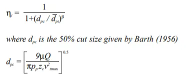
The logistic model developed by Iozia and Leith (1990) is a modified version of the model developed by Barth (1956), which was developed based on force balance. The model operates under the presumption that a particle that is being carried by the vortex is subjected to the influence of two forces: a centrifugal force denoted by the symbol Z, and a flow resistance denoted by the symbol W. Both the core length, denoted by zc, and the core diameter, denoted by dc, are denoted as

The core length zc and slope parameter expression are the additions that Iozia and Leith made to the original Barth (1956) model. These are derived from the statistical analysis of experimental data of cyclones with a diameter of 0.25 metres. The additions were made by Iozia and Leith. It is possible to derive the collection efficiency I of the particle diameter dpi using the formula:

2) LI AND WANG MODEL :

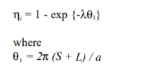
The particle bounce or re-entrainment and turbulent diffusion at the cyclone wall are both accounted for in the model that Li and Wang (1989) developed. An analytical expression of the two-dimensional particle distribution within the cyclone can now be obtained. The following presumptions served as the foundation for the development of Li and Wang's model:

• When it comes to uncollected particles that are contained within the cyclones, the radial particle velocity and the radial concentration profile are not always the same.
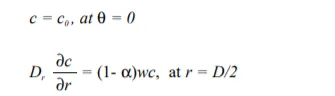
• The following are the boundary conditions that must be met on the cyclone wall in order to account for the turbulent diffusion coefficient and the particle bounce re-entrainment:

• The tangential velocity is related to the radius of cyclone by: uRn = constant.
• The concentration distribution in a cyclone is given as:

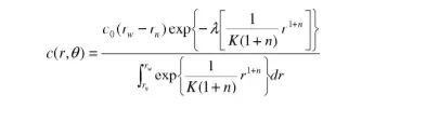
The final form of the expression for the collection efficiency for particles of my size is as follows:

3) KOCH AND LICHT MODEL :

• The collection theory proposed by Koch and Licht (1977) acknowledged both the inherently turbulent nature of cyclones and the distribution of gas residence times within the cyclone. Koch and Licht make the additional following assumptions in their description of the motion of particles in the entry and collection regions:
• The tangential velocity of a particle is identical to the tangential velocity of the flow of gas, which means that there is no difference in the tangential direction between the particle and the flow of gas.
  uRn = constant illustrates the relationship between the tangential velocity and the radius of the cyclone.
• The grade efficiency, denoted by η_i can be calculated using a force balance and an equation based on the particles collection.

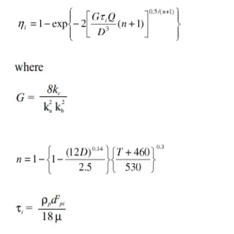
• G is a factor related to the configuration of the cyclone, n isrelated to the vortex and τ is the relaxation term.

4) LAPPLE MODEL :

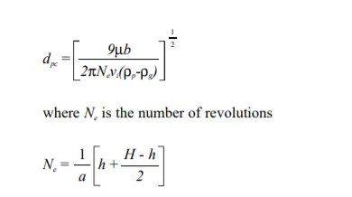
Lapple's model from 1951 was made based on force balance, without taking flow resistance into account. Lapple thought that a particle going into a cyclone would be spread out evenly across the opening. The cyclone collects 50% of the particles that move from the half width of the inlet to the wall. Lapple (1951) came up with a semi-empirical way to figure out the 50% cut diameter (dpc):

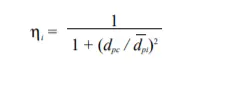
The efficiency of collection of any size of particle is given by

Under room temperature, the Li and Wang model does a great job of predicting how well a cyclone will work. The experimental data from Ray and Kim and Lee fit the Li and Wang model better. The Lapple, Koch, and Licht models overestimate the efficiency of small particles by a smaller amount than they overestimate the efficiency of large particles. For the range of cyclone sizes D = 0.25–0.4m, the Iozia and Leith logistic model agrees well with experimental data. But it can't accurately predict how well a small cyclone (D 0.1m) will work. Iozia and Leith's model is only good for predicting how well a cyclone will work when its diameter is around 0.25 m. When extreme conditions like very high temperature and pressure are added to the mix, the Lapple model makes a pretty good guess. Under high pressure, the Koch and Licht model gives a good estimate of how well a cyclone will work. While the Lapple model is the most accurate way to predict how well a cyclone will work when the temperature is high.

Methods for Solving and Modeling:

We will solve for the five cases mentioned in the goal. We will use ANSYS Fluent solver to create the fluid volume in geometry and perform structured cartesian CFD mesh with boundary definitions, set up the physics of fluid flow, and run the iterations to get solutions. We will use post processing to understand the data in the form of plots, contours, vectors, streamlines, etc.

we shall study for 5 cases as follows.

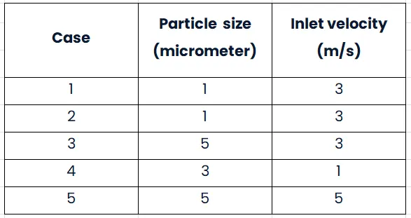
For this kind of problem, we will use the discrete phase option, which lets the user see particles in a fluid medium that are suspended in the fluid. So, we'll look at how well it works and how much the pressure drops at the escape outlet.

We will remember that we are using a student version of ASNYS, so the number of elements we can play with is limited. Then, we add up the results of the case study and compare them with the results of the open literature or book data to prove that the simulation is correct.

Setting up the Preprocessor and the Solver:

Let's open up ANSYS Workbench. To open Fluent flow, you can either drag it into the schematic window or double-click it. The steps in a smooth workflow look like this: GEOMETRY > MESH > SETUP > SOLUTION > RESULTS. Each step must be done before the next one can start.

we will look at case 1 and talk about it in detail,

GEOMETRY >

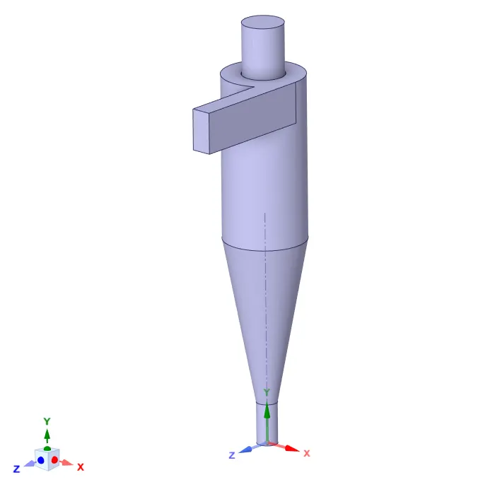
Right-click on the Geometry in the Fluent and choose "New SpaceClaim Geometry." When the space claim application opens, choose FILE > OPEN and then open the Cyclone Separator model.

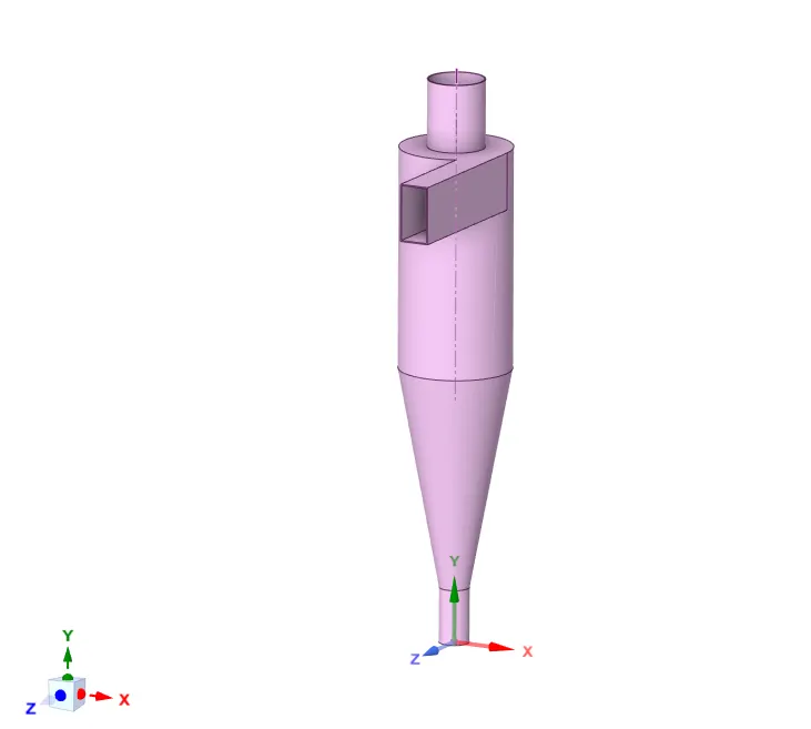
On the Prepare tab, choose the Volume extract option to get the volume of the fluid, and then choose the edges of the inlet and the other two openings to get the volume of the fluid.

We don't need the solid volume to solve the problem, so we can choose "Suppress for physics" to only see the fluid volume in the physics section.

We're ready to go. Once the geometry is done, we can close the space claim and make sure that the fluid flow geometry has been updated, which is shown by a green tick.

MESH >

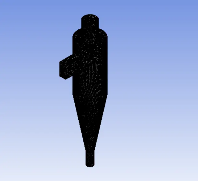
When you right-click on the Mesh and choose "Edit," the Mesh window will appear. The geometry we worked on earlier is already in the Mesh window, so when you click on GENERATE MESH, a mesh should be made automatically.

The size of the mesh here is about 55 mm. The elements are tetra, but we want a structured mesh, so go to Mesh > Methods > Cartesian to change all the tetra elements to structured quad elements. The default size of a mesh element is too big, so we can change it to 5mm. By choosing the Inlet and clicking on N, we will call it the Inlet. The top outlet will be called "outlet escape," and the bottom outlet will be called "outlet trap." If you make changes, you can update the mesh details by clicking on the update icon. If you don't, a sign with a lightning bolt will tell you to update.

When this is done, we should see a green tick near Mesh. The mesh window can be shut.

SETUP >

When you right-click on Setup, the Fluent launcher will open. In the Fluent launcher, choose 3D, Double precision, and the number of cores based on how the user's computer is set up, then click Start.

When you first open the programme, you have to make some choices to set up the simulation. We will choose Type: Pressure-based, Velocity Formulation: Absolute, Time: Steady, and Gravity on in Y axis input -9.81 m/s2. We can turn on viscous and choose k-epsilon > RNG > Swirl dominating flow under the Physics tab.

We will choose air as our default material under "Material."

Injections :

Now we have to specifty the injections of the discrete particles on to the continuous phase.So to do this we have to open injections in the discrete phase modelling.

click on injections -> then create

Particle type : Inert

Material : Anthracite

Injection type : Surface injection

Release from surface : Inlet

In the bottom enable inject using face normal direction

Then in the point properties -> then in that give following values for each variable .

Diameter : 1e-6 m

Velocity magnitude : 3 m/sec

Total flow rate : 1e-20 kg/sec

• Then click ok and close discrete phase modelling.

Boundary conditions :

Inlet - Velocity inlet

velocity : 3 m/sec

DPM : reflect

Outlet (Escape) - Pressure outlet

Gauge pressure : 0 pa

DPM : Escape

Outlet(Trap) - Pressure outlet

Gauge pressure : 0 pa

DPM : Trap

For swirling flows in Method, change the turbulent kinetic energy to the second order upwind and use the coupled method. Let's use Standard initialization compute from inlet.

It's time to begin the simulation now. For Run Calculation, we'll start with 350 iterations and go longer if necessary based on how many particles aren't finished.

We need to export the particle data so that we can analyse it later. To do this, go to File > Export > Particle history data, choose the directory where the data should go, and click write.

In the Outline view of Simulation Reports, clicking on the Report Outline > Generate button should make an Ansys Fluent Simulation Report with all the information about the simulation. This can also be sent as a PDF. We've finished setting up, so you can close the setup.

SOLUTION >

Since some of the solution is worked out in the setup, we can see the green ticks in both the setup and the solution.

RESULTS >

If you right click on the Results, the Post processor should open. The default view is a wireframe model. To see the contour, we can make a plane in the XY plane. All contours and plots can be made here, just like in setup and solution. We can also make an animation of the velocity contour by clicking AUTOSAVE during the solution, then clicking ANIMATE, making a movie, and saving it where we want.

For Cases 2–5, we can change the inlet velocity in the Inlet boundary condition and the DPM. Otherwise, all the steps are the same as in Case 1.

RESULTS:

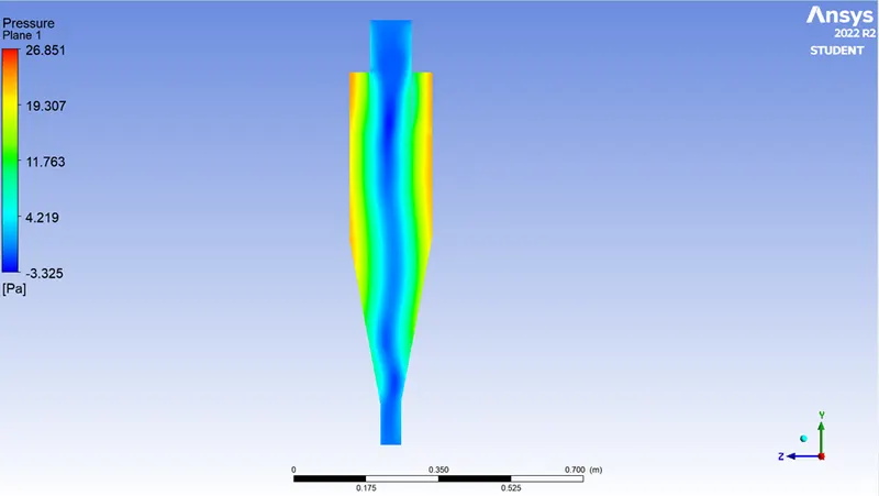
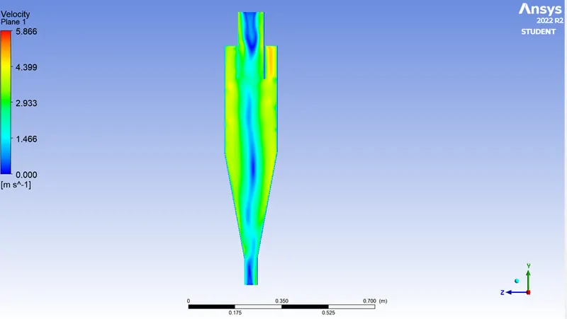
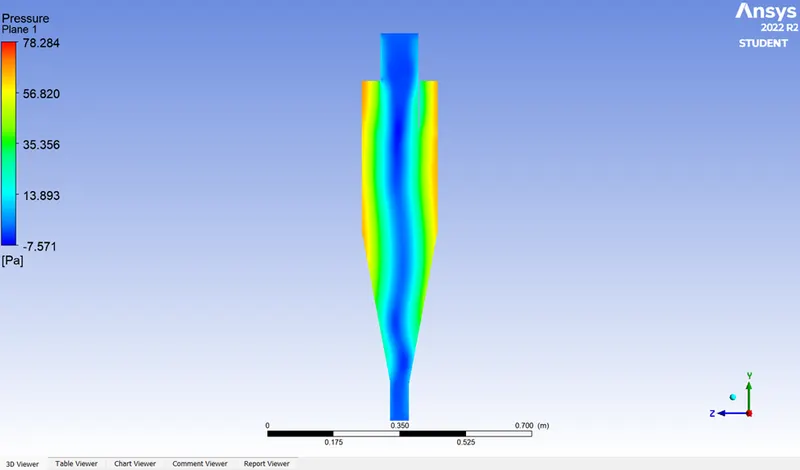
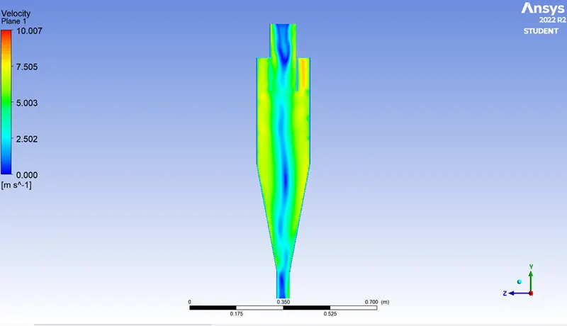
After simulating all of the cases from aim in the same way, we now have a lot of data to compare and study. We'll put all of the contours, plots, and vectors in order so we can compare them and draw a conclusion. Here, only the results of all the cases are shown. Inferences and interpretations will be briefly talked about at the end.

ANIMATIONS :

Case 1 Animation of anthracite particle time

Case 2 Animation of anthracite particle time

Case 3 Animation of anthracite particle time

Case 4 Animation of anthracite particle time

Case 5 Animation of anthracite particle time

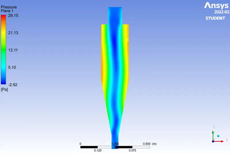
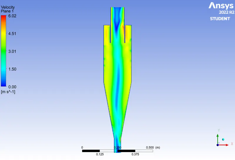
Case 1 - Pressure and Velocity Contour

Case 2 - Pressure and Velocity Contour

Case 3 - Pressure and Velocity Contour

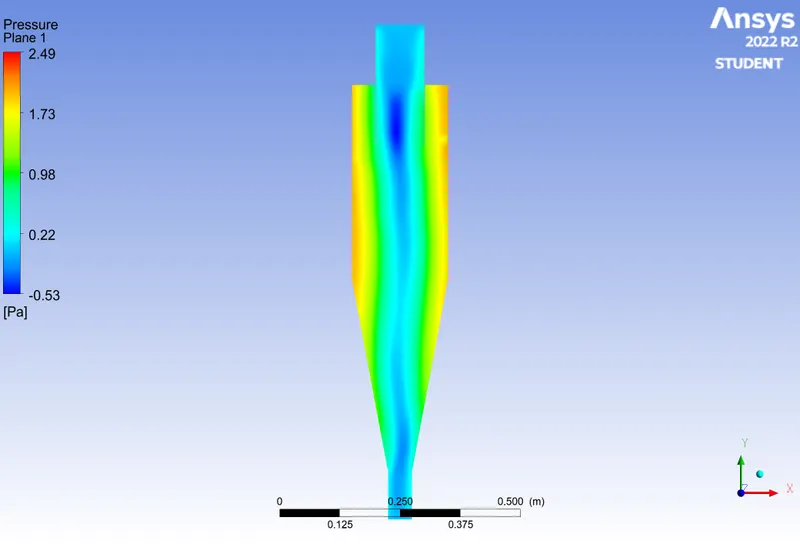
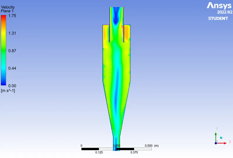
Case 4 - Pressure and Velocity Contour

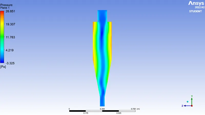
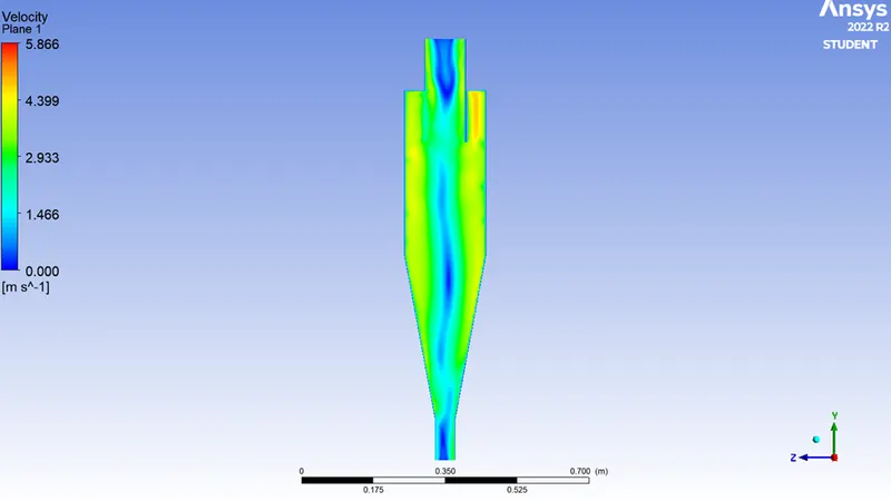
Case 5 - Pressure and Velocity Contour

CONCLUSION:

• The comparison of the 5 cases shows us different data on the pressure and velocity contours, and the animation of the particle data shows us the formation of double vortices, with one vortex pulling the heavy particles down and the other pulling the lighter fluid out of the outlet.
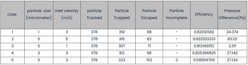
• How well a cyclone separator works is shown by the number of particles it catches compared to the number of particles it doesn't catch. The number of mesh elements in the inlet face is equal to the number of particles that can be tracked, so if we need to study more particles, we can try making the mesh smaller.
• In our case, 378 particles have been tracked. Also, the difference in pressure (Pressure drop) between the inlet and the escape outlet is studied and shown in the table below.
• 

INFERENCES:

Here, we know from the literature that the efficiency is better when the particle size is more than 10 micrometres and is close to 99%. Inferring the same thing from our study, we could see that the efficiency is around 80% in all cases except for the 3 m/s and 5 micrometre particle.

The centrifugal force makes the speed go up around the inlet, and the animation of particle data shows that some particles lose speed as they move down the swirling tube. In real time, this happens because the wall and the speed of the particles rub against each other. So, the cyclone separator can get worn on the inside. If the particles are very small and the speed is optimised for efficiency, cyclone separators are a cheap and effective way to separate them from the fluid medium, whether it's air or water. Also, the size and shape of the cyclone separator play a big role in how the vortex forms.

References:

https://www.sciencedirect.com/science/article/pii/S0307904X06000291

https://www.sciencedirect.com/topics/engineering/cyclone-separator