Week 8 - Simulating Cyclone separator with Discrete Phase Modelling

Week 8 - Simulating Cyclone separator with Discrete Phase Modelling.

Aim:

To perform analysis on cyclone separator and calculate the separation efficiency and pressure drop. Perform velocity versus particle size study from 1 m/s to 5m/s and for particle size from 1 micrometer to 5 micrometer. Tabulate the results and compare for efficiency.

Introduction:

A widely used type of dust-collection equipment is the cyclone separator. A cyclone is essentially a settling chamber in which gravitational acceleration is replaced by centrifugal acceleration. Dust-laden air or gas enters a cylindrical or conical chamber tangentially at one or more points and leaves through a central opening. The dust particles, by virtue of their inertia, tend to move toward the outside separator wall from where they are led into a receiver. Under common operating conditions, the centrifugal separating force or acceleration may range from five times gravity in very large diameter, low-resistance cyclones to 2500 times gravity in very small, high-resistance units.

Within the range of their performance capabilities, cyclones are one of the least expensive dust-collection systems. Their major limitation is that, unless very small units are used, efficiency is low for particles smaller than five microns.

The cyclone separator is a device for separating solid particles from contaminated gas streams, and has long been used in industrial applications such as power generations, gas turbines, chemical processes and so forth. The highly swirling flow field inside a cyclone is very complex, including the interactions between the particulate and fluid phases. Although a lot of empirical theories for estimating the performance of cyclones have been developed so far, these models strongly depend on the experiments that were used to develop the model equations and are not successful for a wide variety of cyclones. Some numerical studies for predicting the cyclone performance have been also carried out recently. However, the interactions between the particulate and fluid phases were not considered in these approaches, and that leads to poor predictions for cases with moderate and high particle concentrations.

Empirical models for Cyclone Separator Efficiency:

• Iozia and Leith Model:

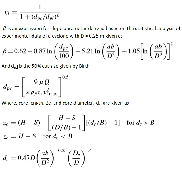
Iozia and Leith logistic Model is a modified version of Barth (1956) model which is developed based on force balance. The model assumes that a particle carried by the vortex endures the influence of two forces: a centrifugal force Z, and flow resistance, W.

The collection efficiency _i of particle diameter d_pi can be calculated by

• Li and Wang Model:

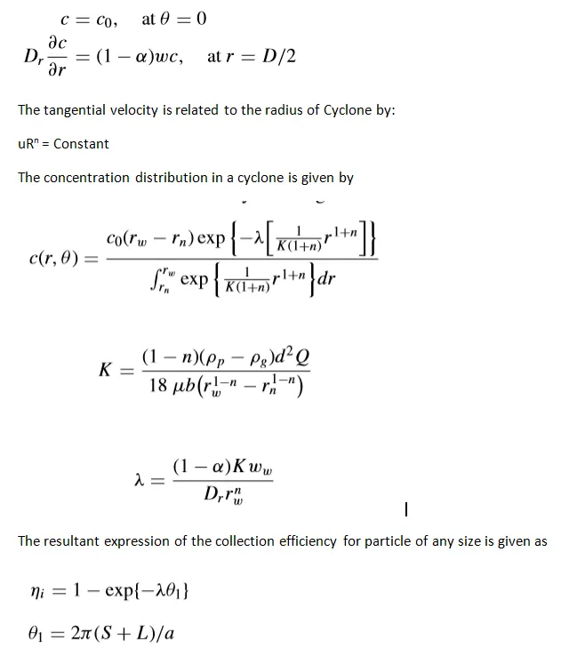
The Li and Wang model include particle bounce or re-entrainment and turbulent diffusion at the cyclone wall. A two-dimensional analytical expression of particle distribution in the cyclone is obtained. Li and Wang model was developed based on the following assumptions:

1. The radial particle velocity and the radial concentration profile are not constant, for uncollected particles within the cyclones.
2. Boundary conditions with the consideration of turbulent diffusion coefficient and particle bounce re-entrainment on the cyclone wall are:

• Koch and Licht Model:

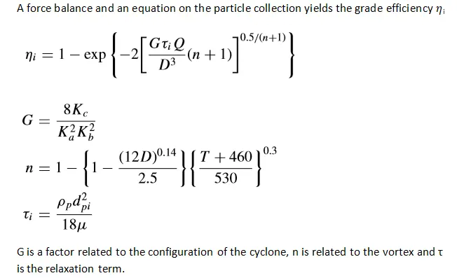
Koch and Licht collection theory recognized the inherently turbulent nature of cyclones and the distribution of gas residence times within the cyclone.

Koch and Licht describe particle motion in the entry and collection regions with the additional following assumptions:

1. The tangential velocity of a particle is equal to the tangential velocity of the gas flow, i.e. there is no slip in the tangential direction between the particle and the gas.
2. The tangential velocity is related to the radius of cyclone by uRⁿ =constant.

• Lapple Model:

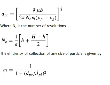
Lapple model was developed based on force balance without considering the flow resistance. Lapple assumed that a particle entering the cyclone is evenly distributed across the inlet opening. The particle that travels from inlet half-width to the wall in the cyclone is collected with 50% efficiency. The semi-empirical relationship developed by Lapple to calculate a 50% cut diameter, d_pc , is

Solving and Modeling approach:

We shall solve for 5 cases as discussed in Aim.We will be using ANSYS Fluent solver to create the fluid volume in geometry and perform structured cartesian CFD mesh with boundary definitions, setup the physics of fluid flow and run the iterations to get solutions, using post processing to interpret the data in form of plots,contours, vectors, streamlines etc.,

we shall study for 5 cases as follows.

Case	Inlet velocity (m/s)	Particle size (micrometer)
1	1	5
2	3	1
3	3	3
4	3	5
5	5	5

For this type of problem, we will be using discrete phase option that allows user to visualize suspended particle in a fluid medium. So, we shall study fo efficiency and the pressure drop at escape outlet.

We shall keep in mind we are using a student version of ASNYS, so we are limited with the number of elements to play with. Then, we tabulate the case study results and compare it with the open literature or book data results to validate the simulation.

Preprocessing and Solver setting:

Let us open ANSYS workbench, now opening Fluent flow can be done by drag and drop in the schematic window or by double clicking on Fluent. The fluent workflow is in a series of steps such as GEOMETRY > MESH > SETUP > SOLUTION > RESULTS. Each step has to be completed for the next step to initialize.

we shall consider case 1 and discuss in detail,

GEOMETRY >

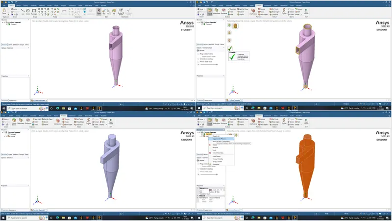
In the Fluent, right click on the Geometry and select New SpaceClaim Geometry. The space claim application opens, select FILE > OPEN and open the Cyclone Separator model.

In the Prepare tab, select the Volume extract option to extract the fluid volume and select the edges if inlet and other two openings to extract the fluid volume.

We don’t need the solid volume for the solving, so we can select the suppress for physics option to see only fluid volume in physics.

We are good to go now. Once the geometry is ready, we can close space claim and check that the fluid flow (fluent) geometry is updated indicated by a green tick.

MESH >

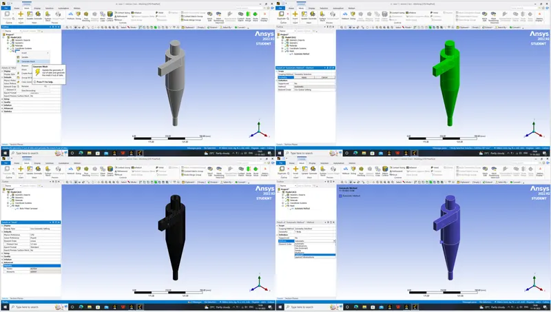
Right clicking on the Mesh and selecting edit opens the Mesh window. Mesh window is preloaded with the geometry we have worked on earlier, so clicking on the GENERATE MESH should create a mesh automatically.

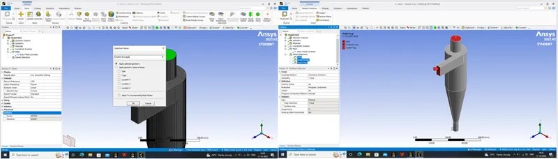
The default mesh size here is 55 mm approx. The elements are tetra, we are interested in structured mesh so go to Mesh > Methods > Cartesian to change all the elements to structured quad elements. The default mesh element size is too large, so we can reduce the element size to 5mm. Selecting the Inlet and clicking on N and we shall name as inlet and name top outlet as outlet escape, bottom outlet as outlet trap respectively. Any changes made, click on the update icon to update the mesh details or else there is an indication of a thunderbolt sign asking the user to update.

Once this is done, we should see a green tick near Mesh. we can close the mesh window.

SETUP >

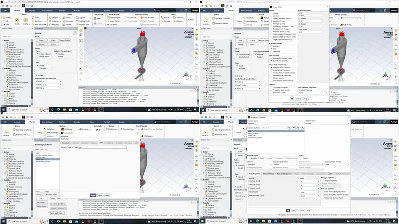
Right clicking on the Setup, opens the Fluent launcher. In the Fluent launcher select 3D, Double precision and select the number of cores as per the user system configuration and click on start.

Upon opening, there are some selections to be done to define the simulation definitions, we shall select Type: Pressure based, Velocity Formulation: Absolute, Time: Steady, Gravity on in Y axis input -9.81 m/s^2. Under the Physics tab, we can turn on viscous and select k-epsilon > RNG > Swirl dominating flow as well.

Under the materials we shall select air as our default material.

In the Discrete phase deck, select Injections > Create > Injection type surface and select the inlet surface. And input X velocity as 3 m/s (as per case) and the material is anthracite by default. The particle size can be input as 0.000005 m (as per case).

In the Boundary conditions, select the inlet as velocity inlet and in DPM as Inlet. Let the fluid volume be wall with DPM as reflect, Outlet escape as escape, outlet trap as trap.

In Method, for the swirl dominating flows change the turbulent kinetic energy to second order upwind, and coupled method. Let us use Standard initialization compute from inlet.

Now, it's time to start the simulation. For Run Calculation, we shall run for 350 iterations initially if required we shall extend based on the number of incomplete particles.

We need to export the particle data for us to analyse in post processing, for that go to File > Export > Particle history data and select the required directory and click write.

In the Outline view under Simulation Reports, clicking on the Report Outline > Generate should generate a Ansys Fluent Simulation Report which is automatically generated with all the information of the simulation in it. This can be exported as a PDF also. We are done with setup, we can close the setup.

SOLUTION >

Since some solution is calculated in the setup itself, we can see the green ticks in both setup and solution too.

RESULTS >

Right clicking on the Results should open the Post processor. Default view is a wireframe model, we can create a plane in XY to view contour. Similar to setup and solution, all contours and plots can be created here, in addition to that we can create an animation of the velocity contour by clicking on AUTOSAVE during the solution and clicking on ANIMATE select make movie and save in desired location.

For Case 2 to 5 we can change the inlet velocity in Inlet boundary condition and in DPM otherwise all steps are same as case 1.

RESULTS:

After repeating the similar manner of simulation procedures for all cases from aim, we have a handful of data to compare and study. We shall put in order all the contours, plots and vectors for us to compare and come to a conclusion. Here, only the results of all cases are displayed, its inference and interpretation shall be discussed briefly in conclusion.

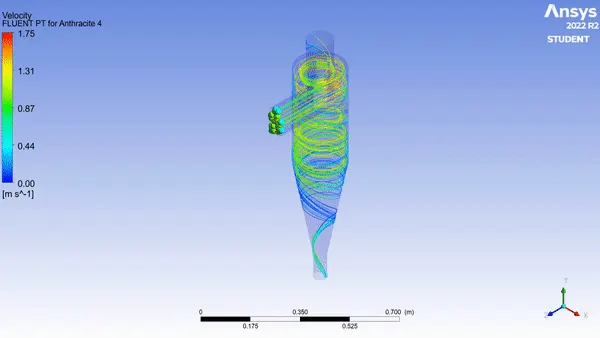
Case 1 - Velocity Tracking data

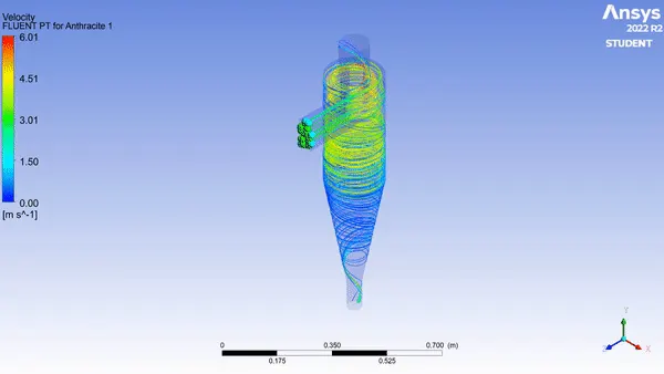
Case 2 - Velocity Tracking Data

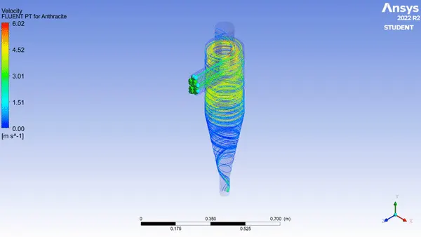
Case 3 - Velocity Tracking data

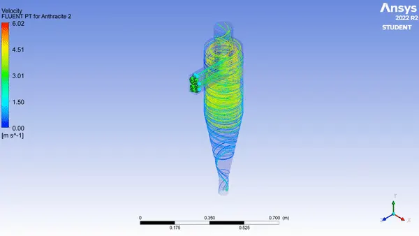
Case 4 - Velocity Tracking data

Case 5 - Velocity Tracking data

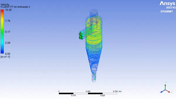
Case 1 - Pressure and Velocity Contour

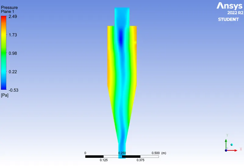
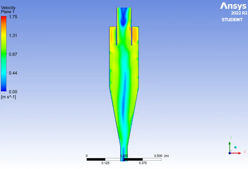
Case 2 - Pressure and Velocity Contour

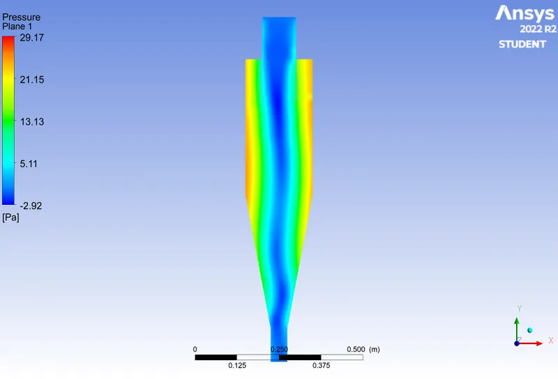
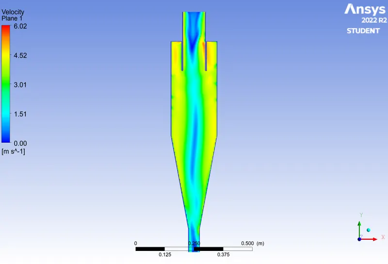
Case 3 - Pressure and Velocity Contour

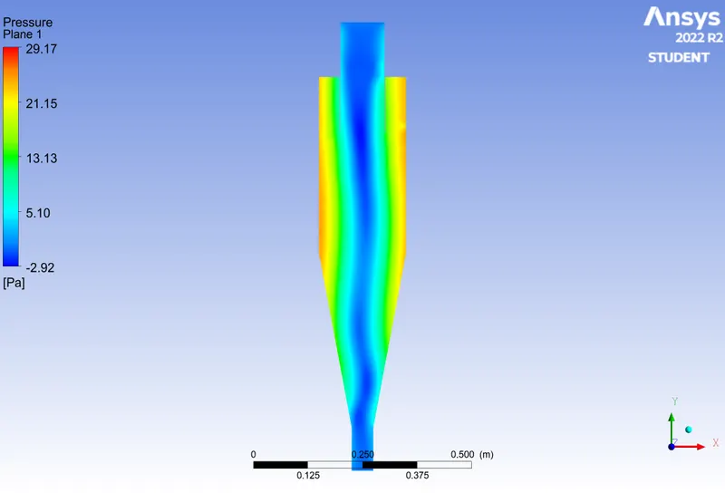
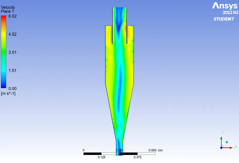
Case 4 - Pressure and Velocity Contour

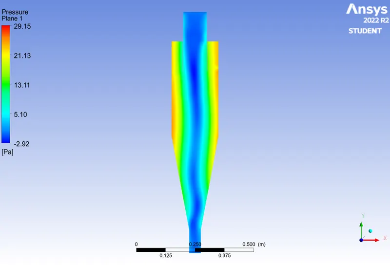
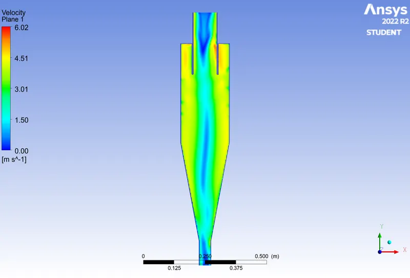
Case 5 - Pressure and Velocity Contour

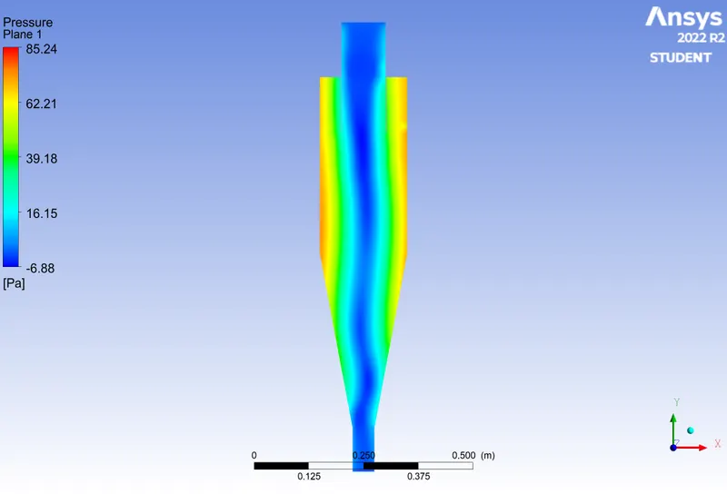
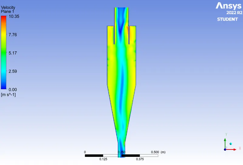
CONCLUSION:

The 5 case comparison shows us various data on pressure and velocity contour and the animation of the particle data shows us the formation of double vortices one leading the heavy suspended particles downward and the inner vortex leading the lighter fluid to escape outlet.

The efficiency of the cyclone separator is the ratio of the number of particles trapped to the number of particle tracked. The number of particles tracked is the number of mesh elements in the inlet face, so if we need to study more quantity of particles try reducing the mesh size.

In our case the number of particles tracked is 378. Also the pressure difference (Pressure drop) between the inlet and the escape outlet is also studied and tabulated as follows,

case	inlet velocity (m/s)	particle size (micrometer)	particle Tracked	Particle Trapped	Particle Escaped	Particle Incomplete	Efficiency (%)	Pressure Difference(Pa)
1	1	5	378	307	71	-	81.22	2.27
2	3	1	378	310	68	-	82.01	25.36
3	3	3	378	312	66	-	82.54	27.05
4	3	5	378	223	152	3	58.99	27.08
5	5	5	378	315	63	-	83.33	83.1

INFERENCES:

Here, with reference from the literatures we come to know that the efficiency is better close to 99% when the particle size is more than 10 micrometer. The same is inferred in our study too, we could see that the efficiency is around 80% for all cases except for the 3 m/s and 5 micrometer particle.

Velocity increases around the inlet due to the centrifugal action, and the animation of particle data shows that some particles loose its velocity as it moves down swirling. In real time, this occurs due to the friction between the wall and the particle velocity. So, the cyclone separator is prone to internal wear. Otherwise if the particle size is very small with a optimized velocity for efficiency, cyclone separators are economic and efficient devices for separating suspended particles from the fluid medium, be it air or liquid. Also, the cyclone separator vortex formation greatly depends on the dimensions of the geometry as well.

References:

EVALUATION ON EMPIRICAL MODELS FOR THE PREDICTION OF CYCLONE EFFICIENCY

Jolius Gimbun1 , T.G. Chuah2 , Thomas S. Y. Choong2 and A. Fakhru’l-Razi2
1Faculty of Chemical and Natural Resources Engineering, University Collage of Engineering and Technology Malaysia,
KUKTEM, Bandar MEC, 25200 Kuantan, Pahang
2Department of Chemical and Environmental Engineering, Faculty of Engineering, Universiti Putra Malaysia,
43400 UPM, Serdang, Selangor

https://www.sciencedirect.com/topics/engineering/cyclone-separator

https://www.sciencedirect.com/science/article/pii/S0307904X06000291

https://www.researchgate.net/publication/232747389_A_CFD_Study_on_the_Prediction_of_Cyclone_Collection_Efficiency